Chapter 23 Samples from a normal distribution

This text (roughly) follows Chapter 11 of our textbook. The reading below is required, Whitlock and Schluter (2020) is not.

Motivating scenarios: We have a normally distributed sample so we have an estimate of its standard deviation, not the true parameter. How do we estimate uncertainty and test hypotheses in this case? Or we have a linear model and want to understand the common test statistic $t$.

Learning goals: By the end of this chapter you should be able to

Describe the difference between the standard normal distribution ($Z$), and the $t$ distribution.
Simply explain a $t$ value.
Use the $t$ distribution to find the 95% confidence interval for a sample from the normal distribution.
Test the null hypothesis that a sample mean comes from a population with some parameter value.
- For a one-sample t-test.
- For a paired t-test.
Use the _t() family of functions to
- Calculate the probability of finding a value more extreme than some number of interest from a specified $t$ distribution pt(), and
- Find a specified quantile of a $t$ distribution with qt().

23.1 The dilema and the solution

The dilema

In Chapter 22 we saw a bunch of useful math for samples from a normal distribution. Importantly, we saw that by Z-transformation ($Z = \frac{x-\mu}{\sigma}$ for one obervation, or $Z = \frac{\overline{x}-\mu}{\sigma / \sqrt{n}}$ for the mean of a sample of size $n$) we can meaningfully summarize values as their distance, in standard deviations, away from the population mean.

But, their is one problem here. We usually have a sample estimate of the standard deviation $s$, not its true population parameter, $\sigma$. Because of this, the standard normal distribution (aka the Z distribution) is not quite right (although it is almost right), because it does not incorporate uncertainty in our estimate of the standard deviation.

The solution

The solution to this dilemma is to use a sampling distribution, called the t-distribution, that includes uncertainty in our estimate of the standard deviation. There are many t-distributions – each associated with some numbers of degrees of freedom (remember this is the number of observations whose values can vary before you know them all).

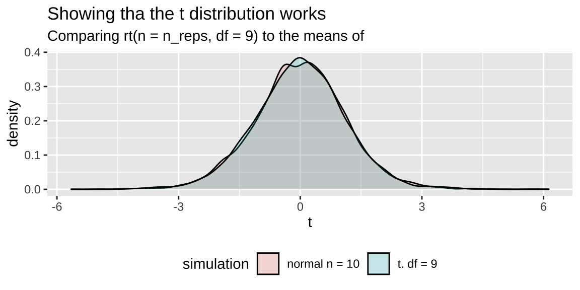
A t-distribution looks a lot like the standard normal distribution, however, the tails are “fatter” to model the possibility that we underestimated $s$. As our sample (and therefore our degrees of freedom) gets larger, the t distribution gets closer and closer to the standard normal distribution (Fig 23.1) because our confidence in the estimate of the standard deviation increases.

Figure 23.1: Comparing the t (black) and standard normal (Z, red) distributions for different degrees of freedom.

23.2 t is a common test statistic

Because most sampling distributions are normal, but we almost never know the true population standard deviation, we deal with t-values a lot in statistics. Every time we see a t-value, t is the number of standard errors away our estimate is from its hypothesized parameter under the null hypothesis. We will see t values as a test stat in basically every linear model so get used to them! Here we introduce this statistic by considering a single sample.

23.3 Calculations for a t-distribution

23.3.1 Calculating t

Like the Z-distribution for a sample mean, the t-value describes the number of standard errors between our sample mean and the population parameter. The math for calculating a t-value is basically the same as for a Z value – we find the difference between our sample estimate, $\overline{x}$, and the hypothesized population parameter, $\mu_0$, and divide that by the sample standard error, $s/\sqrt{n}$.

\[t = \frac{\overline{x}-\mu_0}{SE_x} = \frac{\overline{x}-\mu_0}{s/\sqrt{n}}\]

23.3.2 Calcualting the degrees of freedom

The number of degrees of freedom describes how many individual values we need to know after building our model of interest, before we know every data point.

For example, if you have a sample of size

$n = 1$, and I tell you the sample mean, you know every data point, and there are zero degrees of freedom.
$n = 2$, and I tell you the sample mean, you need one more data point to fill in the rest, and there is one degree of freedom.
$n = 3$, and I tell you the sample mean, you need two more data points to fill in the rest, and there are two degrees of freedom.

So, when we are estimating a sample mean $\overline{x}$, the degrees of freedom equals the sample size minus one. $df = n-1$.

23.3.3 Calculating a confidence interval

We use the t-distribution to find the $1-\alpha$% confidence interval for the estimated mean of a sample from a normal distribution.

To estimate the upper (or lower) $1-\alpha$ confidence intervals, we take our estimate and add (or subtract) the product of the sample standard error and the critical value which separates the middle $1-\alpha$ of the distribution from the rest of the distribution. This makes sense because this should contain 95% of sample means estimated from a population.

\[\begin{equation} \begin{split} (1-\alpha)\%\text{ CI } &= \overline{x} \pm t_{\alpha/2} \times SE_x\\ &= \overline{x} \pm t_{\alpha/2} \times s_x / \sqrt{n} \end{split} \tag{23.1} \end{equation}\]

Where $t_{\alpha/2}$ is the critical two-tailed t value for a specified $\alpha$ value. We find $t_{\alpha/2}$ in R with the pt() function — $t_{\alpha/2}$ = qt(p = alpha/2, df = 9). Remember that we divide $\alpha$ by two in this calculation to include both sides of the sampling distribution. Figure shows the critical value (two-tailed $\alpha = 0.05$) for a sample from the t-distribution with nine degrees of freedom.

So, for example, we find the lower bound of a 95% confidence interval from a sample of size 10 as

Lower 95% CI with 9 df = $\overline{x} + t_{.05/2,df =9} \times SE_x$

What is $t_{.05/2,df =9}$? From 23.2 it looks to be a bit less than 2.5. Now let’s find out what it is more precisely!

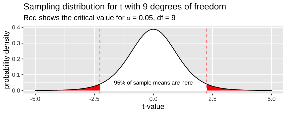
Figure 23.2: The sampling distribution for t with nine degrees of freedom. Area in with is the middle 95% of the distribution

Finding the critical value in R

If you have taken stats elsewhere, you probably remember statistical tables you used for looking up critical values. R has these built in with the q_ (for quantile) family of functions. For example if we had a sample of size 10, qt(p = .025, df = 10 - 1, lower.tail = FALSE) will find the t value that separates the upper (because lower.tail = FALSE) 97.5% of the distribution from the rest.

Returning to our example, above, we find the lower bound of a 95% confidence interval from a sample of size 10 as

Lower 95% CI with 9 df = $\overline{x} + t_{.05/2} \times SE_x$
Lower 95% CI with 9 df = $\overline{x} +$ qt(p = .05/2, df = 9) $\times s_x / \sqrt{10-1}$
Lower 95% CI with 9 df = $\overline{x} +$ -2.262 $\times s_x / 3$.

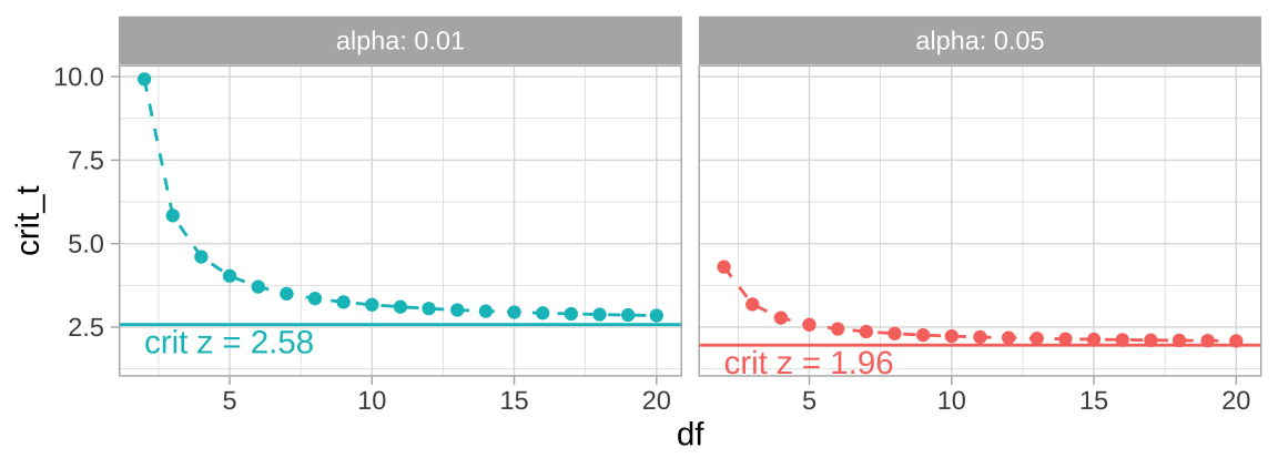
The code below will find and plot the critical t-value for two tail 95 and 99 percent confidence intervals across a range of values for the degrees of freedom.

23.3.4 Calculating a p-value

Remember the p-value is the probability that a random sample from the null distribution would have a test statistic as or more extreme than the test statistic that we observed.

So, let’s say we had a sample of size 10 and calculated a t value of -1.5. We would find where on the sampling distribution our test statistic is, and integrate the area from there to $-\infty$ on the sampling distribution of $t$ with nine degrees of freedom, and multiply this be two to get both tails of the distribution (i.e. the area of the blue region in Figure 23.3).

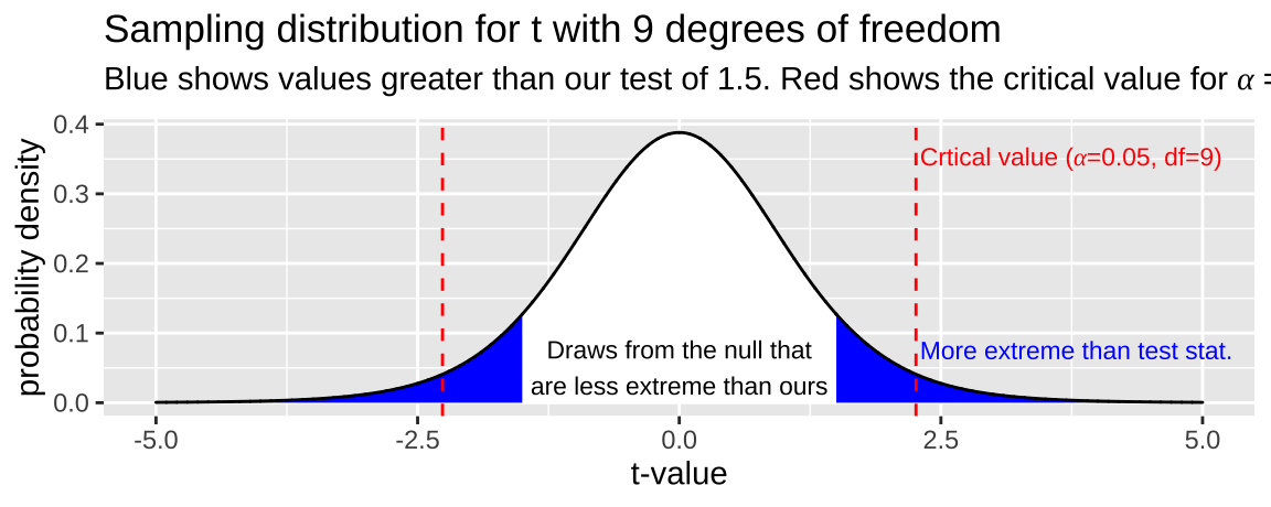
The sampling distribution for *t* with nine degrees of freedom. Area in blue is as or more extreme than the test statitic, -1.5. Red lines show the critical value

Figure 23.3: The sampling distribution for t with nine degrees of freedom. Area in blue is as or more extreme than the test statitic, -1.5. Red lines show the critical value

While I can’t integrate well by eye (I would guess blue integrates to 0.2), this value is clearly not a particularly unexpected outcome – $p >\alpha$ so we fail to reject the null hypothesis.

Calculating a p-value in R with `pt()`

We can use the pt() function to find the probability that a random sample from the t distribution has a test statistic as or more than ours. In doing so, be sure to look at both sides!

df         <- 9 
observed_t <- 1.5
p_val      <- 2 * pt(q = observed_t, df = df, lower.tail = FALSE)

The code above returns a p-value of p_val %>% round(digits = 3), consistent with our visual estimate above. So we fail to reject the null hypothesis.

23.3.5 Calculating the effect size

The t is useful for hypothesis testing and including uncertainty in our estimnaes, but it does not describe the size of the effect. A simple measure of the effect size, known as Cohen’s d, is the number of standard deviations away from the null mean our estimate is

\[\text{Cohen's d} = \frac{\overline{x}-\mu_0}{s_x}\].

23.4 Assumptions of the t-distribution

The t-distribution assumes that

Data are collected without bias
Data are independent
The mean is a meaningful summary of the data
Samples (or more particularly, the sampling distribution) are normal

23.4.1 What to do when we violate assumptions

As always, bias is very hard to deal with, and is best addressed by a better study.
Non independent data can be modeled, but such models are beyond the scope of this chapter.
Whether the mean is a meaningful summary or not is a biological question.

The normality assumption is easiest to deal with. If we violate this assumption we can:
- Ignore it (if the violation is minor) because the central limit theorem is there for us. OR
- Transform the data to an appropriate scale OR
- Bootstrap to estimate uncertainty and/or conduct a binomial test, with numbers greater than $mu_0$ as “successed” and less than $\mu_0$ as “failures.”

23.5 Example of a one sample t-test

Has Climate Change Moved Species Uphill?

A common use of the t-distribution is to test the null hypothesis that the mean takes some value. This is called a one sample t-test.

For example, Chen et al. (2011) wanted to test the idea that organisms move to higher elevation as the climate warms. To test this, they collected data from 31 species, plotted below (Fig 23.4).

range_shift_file <- "https://whitlockschluter3e.zoology.ubc.ca/Data/chapter11/chap11q01RangeShiftsWithClimateChange.csv"
range_shift <- read_csv(range_shift_file) %>%
  mutate(x = "", uphill = elevationalRangeShift > 0)

ggplot(range_shift, aes(x = x, y = elevationalRangeShift))+
  geom_jitter(aes(color = uphill), width = .05, height = 0, size = 2, alpha = .7)+
  geom_hline(yintercept = 0, lty= 2)+
  stat_summary(fun.data = "mean_cl_normal") + 
  theme(axis.title.x = element_blank())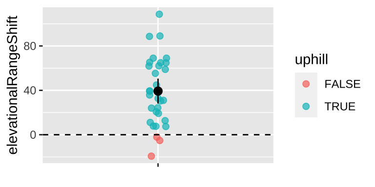

Change in the elevation of 31 species. Data from @Chen2011.

Figure 23.4: Change in the elevation of 31 species. Data from Chen et al. (2011).

23.5.1 Estimation

The first step is to summarize the data. Let’s calculate the mean, sample size, standard deviation and Cohen’s D (assumin $\mu_0$ = 0).

mu_0 <- 0
range_shift_summary  <- range_shift %>%
  summarise(n = n(), 
            this_mean = mean(elevationalRangeShift),
            this_sd   = sd(elevationalRangeShift ),
            cohens_d = (this_mean - mu_0) / this_sd)

n	this_mean	this_sd	cohens_d
31	39.33	30.66	1.28

So we see ranges have shifted upwards – about 39.3 meters, which is more than one standard deviation in the change in elevation across species.

23.5.2 Evaluating assumptions

library(plotly)
range_data <- range_shift %>%
  separate(col = "taxonAndLocation", into = c("taxon","location"), sep = "_") %>%
  ggplot(aes(x = location , fill = taxon))+
  geom_bar()+
  coord_flip()
ggplotly(range_data) # to allow readers to engage with the data

Figure 23.5: Taxa and locality information from Chen et al. (2011)

Are date biased? I hope not, but it would depend on aspects of study design etc. For example, we might want to know if species had as much area to increase in elevation as to decrease etc…. How were species picked….
Are Data independent? Check out the data above. My sense is that they aren’t all independent. So much data is from the UK (Figure 23.5). What if there is something specific about low elevation regions in the UK? Anyways, I wouldn’t call this a reason to stop the analysis, but it is a good thing to consider.
Is the mean a meaningful summary of the data? My sense is yes, but look for yourself!
Are samples (or more particularly, the sampling distribution) normal? My sense is yes, but look for yourself!

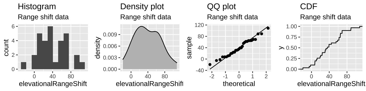
The distribution of range shifts in the @Chen2011 data.

Figure 23.6: The distribution of range shifts in the Chen et al. (2011) data.

So it looks like we’re ready to move on! But we should probably worry some about nonindependence.

23.5.3 Uncertainty

We can estimate this uncertainty in this estimate of range shift by a bootstrap or by using the formulae above.

Bootstrap based estimates of uncertainty

As we have done before, we can fake a sampling distribution by resampling from our data with replacement many times and estimate uncertainty as the variability in this sampling distribution

n_reps <- 50000
range_shift   %>%
  rep_sample_n(size = nrow(range_shift ), replace = TRUE, reps = n_reps)     %>%
  summarise(mean_vals = mean(elevationalRangeShift)) %>%
  summarise(se = sd(mean_vals),
            lower_95CI = quantile(mean_vals, prob = 0.025),
            upper_95CI = quantile(mean_vals, prob = 0.975))

## [38;5;246m# A tibble: 1 x 3[39m
##      se lower_95CI upper_95CI
##   [3m[38;5;246m<dbl>[39m[23m      [3m[38;5;246m<dbl>[39m[23m      [3m[38;5;246m<dbl>[39m[23m
## [38;5;250m1[39m  5.45       28.8       50.1

t based estimates of uncertainty

Alternatively, we can approximate a sampling distribution by using the t-distribution. Remember that the standard error of the normal is $\frac{s}{\sqrt{n}}$:

alpha      <- 0.05

range_shift_summary %>%
  mutate(se = this_sd / sqrt(n),
         lower_95CI = this_mean + se * qt(p = alpha/2, df = n-1, lower.tail = TRUE),
         upper_95CI = this_mean + se * qt(p = alpha/2, df = n-1, lower.tail = FALSE)) %>%
  dplyr::select( se, lower_95CI, upper_95CI)

## [38;5;246m# A tibble: 1 x 3[39m
##      se lower_95CI upper_95CI
##   [3m[38;5;246m<dbl>[39m[23m      [3m[38;5;246m<dbl>[39m[23m      [3m[38;5;246m<dbl>[39m[23m
## [38;5;250m1[39m  5.51       28.1       50.6

Reassuringly, these values are pretty close to what we found by bootstrapping.

23.5.4 Hypothesis testing

Let’s lay out the null and alternative hypotheses:

$H_0:$ On average organisms have not increased or decreased their elevation.
$H_A:$ On average organisms have increased or decreased their elevation.

How to test this null? tbh I have a hard time thinking of how to permute, so let’s use the t-distribution tricks!

Calculations for hypothesis testing in R

First, let’s calculate $t=\frac{\overline{x}-\mu_0}{se_x}$, and then look up the p-value with pt(), remembering to multiply it by two to get both tails of the distribution.

mu_0 <- 0 # null hypothesis, zero change

range_shift_summary %>%
  mutate(df = n - 1,
         se =  this_sd / sqrt(n),
         t  = (this_mean - mu_0) / se,
         p_val = 2 * pt(q = abs(t), df = df, lower.tail = FALSE) ) %>%
  dplyr::select(df, t,        p_val)

## [38;5;246m# A tibble: 1 x 3[39m
##      df     t        p_val
##   [3m[38;5;246m<dbl>[39m[23m [3m[38;5;246m<dbl>[39m[23m        [3m[38;5;246m<dbl>[39m[23m
## [38;5;250m1[39m    30  7.14 0.000[4m0[24m[4m0[24m[4m0[24m060[4m6[24m

We find a really small p-value, meaning that the null hypothesis would rarely generate such extreme data. Since p is less than the traditional $\alpha$ threshold we reject the null hypothesis and conclude that ranges have shifted upward.

Note this doesn’t mean the null is wrong, it just means that we’re proceeding as if it is.

Functions for t testing in R

Or, more simply, we could use the t.test() function in R, setting $\mu$ to its proposed value under the null hypothesis.

t.test(x = pull(range_shift, elevationalRangeShift), mu = mu_0)

## 
##  One Sample t-test
## 
## data:  pull(range_shift, elevationalRangeShift)
## t = 7.1413, df = 30, p-value = 6.057e-08
## alternative hypothesis: true mean is not equal to 0
## 95 percent confidence interval:
##  28.08171 50.57635
## sample estimates:
## mean of x 
##  39.32903

Reassuringly, we get the same answer from t.test() as we did from our calculations! We still reject the null! As a bonus, the t.test() function also returns the confidence intervals, which again match our calculations!

Remember that the tidy() function in the broom package cleans up this awkward model output. To show you this, while pushing our concepts forward, let’s run the same test again, but exclude samples from the UK, to minimize the possibility that our results are driven by one over-represented country

library(broom)
range_shift_noUK <- range_shift %>%
  filter(str_detect(taxonAndLocation,"UK", negate = TRUE)) # remove observations from UK
  
t.test(x = pull(range_shift_noUK, elevationalRangeShift), mu = mu_0)  %>%
  tidy()

## [38;5;246m# A tibble: 1 x 8[39m
##   estimate statistic  p.value parameter conf.low conf.high method            alternative
##      [3m[38;5;246m<dbl>[39m[23m     [3m[38;5;246m<dbl>[39m[23m    [3m[38;5;246m<dbl>[39m[23m     [3m[38;5;246m<dbl>[39m[23m    [3m[38;5;246m<dbl>[39m[23m     [3m[38;5;246m<dbl>[39m[23m [3m[38;5;246m<chr>[39m[23m             [3m[38;5;246m<chr>[39m[23m      
## [38;5;250m1[39m     48.6      4.95 0.000[4m2[24m[4m1[24m[4m5[24m        14     27.5      69.7 One Sample t-test two.sided

A sign test for data that don’t meet normality assumptions

Here the data clearly meet assumptions of normality – but what if they didn’t? A common solution is to conduct a sign test. To do so, we count the number of observations greater than the null expectations and conduct a binomial test against the null that numbers greater than and less than the null are equally provable (this is called a sign test).

range_sign <-range_shift %>%
  mutate(sign = sign(elevationalRangeShift - mu_0)) %>%
  filter(sign != 0 ) %>% # remove zeros
  summarise(n = n(), 
            up = sum(sign == 1))

binom.test(x = pull(range_sign , up), n = pull(range_sign , n), p = mu_0)

## 
##  Exact binomial test
## 
## data:  pull(range_sign, up) and pull(range_sign, n)
## number of successes = 28, number of trials = 31, p-value < 2.2e-16
## alternative hypothesis: true probability of success is not equal to 0
## 95 percent confidence interval:
##  0.7424609 0.9795801
## sample estimates:
## probability of success 
##              0.9032258

23.5.5 Conclusion

We find that on average species have shifted their range to higher elevations (a mean of 39.3 meters with a standard error of 2.21 meters and 95% confidence interval between 28.1 and 50.6). There is some variability among species (sd = 30.7), but this variability is overwhelmed by the overall march uphill (Cohen’s d = 1.28). Such an extreme change is an unlikely outcome of the null (t = 7.14, df = 30, p = $6.06 \times 10^{-8}$). This result is not driven by samples from the UK, which make up half the data set – we get a similar result (mean = 48.6, 95% confidence interval between 27.5 and 69.7) after excluding them.

23.6 Paired t-test

A common use of this approach is to look for the difference between groups when there are natural pairs in each group. These pairs should be similar to each other in every way, aside from the difference we are investigating.

Note that we cant just pair up random individuals and call it a paired t-test.

For example, say we were interest to test the idea that more money resulted in more problems. So we gave some people $100,000 and others $1 and then got a quantitative and normally distributed measure of their problems.

If we randomly gave twenty people $100,000 and twenty people $1, we could not just randomly form 20 pairs and do a paired t-test.
But we could pair people by background (eg find a pair of waiters at similar restaurants give one 100k and another $1, then do the same for a pair of professors, and a pair of hairdressers, and a pair of doctors, and a pair of programmers etc… until we ad twenty such pairs) we could then conduct a paired t-test.

23.6.1 Paired t-test example:

Rutte (2007) tested for the existence of “generalized reciprocity” in the Norway rat, Rattus norvegicus. That is, they asked whether a rat that had just been helped by a second rat would be more likely to help a third rat than if it had not been helped. Focal female rats were trained to pull a stick attached to a try that produced food for their partners but not themselves. Subsequently, each focal rat’s experience was manipulated in two treatments. Under one treatment, the rat was helped by three unfamiliar rats (who pulled the appropriate stick). Under the other treatment, focal rats received no help from three unfamiliar rats (who did not pull the appropriate stick). Each focal rat was exposed to both treatments in random order. Afterword, each focal rat’s tendency to pull for an unfamiliar partner rat was measured. The number of pulls in a given period (in pulls/min) by 19 focal female rats after both treatments is available here, and is plotted below.

rat_link <- "http://whitlockschluter.zoology.ubc.ca/wp-content/data/chapter12/chap12q31RatReciprocity.csv"
rat_dat  <- read_csv(rat_link) %>% 
  mutate(help_minus_nohelp = AfterHelp - AfterNoHelp,
         sign = case_when(help_minus_nohelp == 0 ~ "0",
                          help_minus_nohelp >0   ~ "+",
                          help_minus_nohelp <0   ~ "-"))

# Makng some plots!
long_rat <-  rat_dat %>% 
  pivot_longer(cols = contains("Help",ignore.case = FALSE), 
               names_to = "treatment", values_to = "help_other", names_prefix = "After")

ggplot(long_rat,  aes(x = treatment, y = help_other, group = focalRat, color = sign)) +
  geom_point(size = 3, alpha = .4) +
  geom_line(alpha = .5)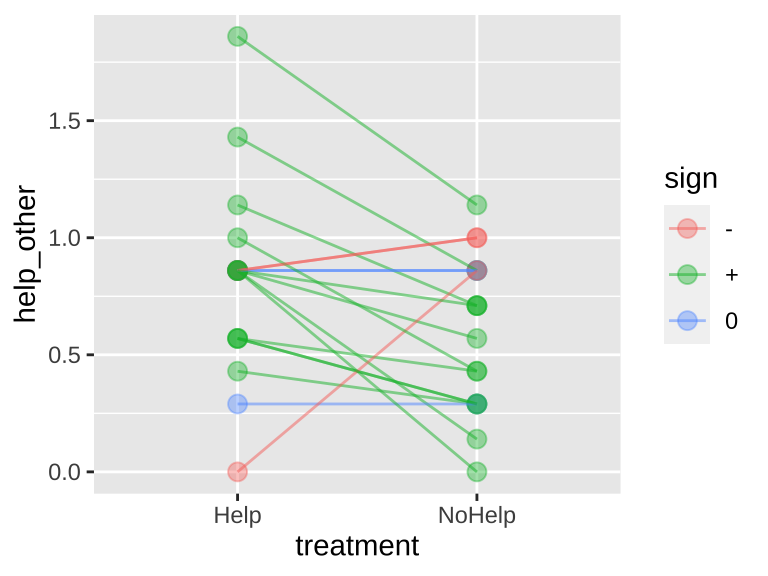

Evidence for generalized reciprocity? Lines connect how helpful individual rats where to others (measured as the number of pulls to give another rat food) when the focal rate did or did not get help themselves. Data from @rutte2007.

Figure 23.7: Evidence for generalized reciprocity? Lines connect how helpful individual rats where to others (measured as the number of pulls to give another rat food) when the focal rate did or did not get help themselves. Data from Rutte (2007).

We can do a paired t-test by running a one-sample t-test on the difference between paired observations of individual rats with a null differnece of zero, as follows

t.test(pull(rat_dat, help_minus_nohelp), mu = 0) %>%tidy()

## [38;5;246m# A tibble: 1 x 8[39m
##   estimate statistic p.value parameter conf.low conf.high method            alternative
##      [3m[38;5;246m<dbl>[39m[23m     [3m[38;5;246m<dbl>[39m[23m   [3m[38;5;246m<dbl>[39m[23m     [3m[38;5;246m<dbl>[39m[23m    [3m[38;5;246m<dbl>[39m[23m     [3m[38;5;246m<dbl>[39m[23m [3m[38;5;246m<chr>[39m[23m             [3m[38;5;246m<chr>[39m[23m      
## [38;5;250m1[39m    0.219      2.42  0.026[4m4[24m        18   0.028[4m7[24m     0.409 One Sample t-test two.sided

Or by telling R to do a paired t test as follows

t.test(pull(rat_dat, AfterHelp),pull(rat_dat, AfterNoHelp), paired = TRUE) %>%tidy()

## [38;5;246m# A tibble: 1 x 8[39m
##   estimate statistic p.value parameter conf.low conf.high method        alternative
##      [3m[38;5;246m<dbl>[39m[23m     [3m[38;5;246m<dbl>[39m[23m   [3m[38;5;246m<dbl>[39m[23m     [3m[38;5;246m<dbl>[39m[23m    [3m[38;5;246m<dbl>[39m[23m     [3m[38;5;246m<dbl>[39m[23m [3m[38;5;246m<chr>[39m[23m         [3m[38;5;246m<chr>[39m[23m      
## [38;5;250m1[39m    0.219      2.42  0.026[4m4[24m        18   0.028[4m7[24m     0.409 Paired t-test two.sided

Either way, we get the exact same thing, and reject the null hypotheses, and conclude that helped rats help more (although we know this could have been a false positive).

23.7 Quiz

23.8 Extra material for the advanced / bored / curious

23.8.1 Likelihood based inference for a sample from the normal

We calculate the likelihoods and do likelihood-based inference for samples from a normal the exact same way as we did previously.

Because this all relies on pretending we are using population parameters. So we calculate the sd as the distance of each data point from the proposed mean, and divide by n rather than n-1.

The big benefits of likelihood-based inference are

Its flexibility. We are doing this for a simple t-test, which we can obviously do without likelihoods. BUT we can use likelihood-based inference for any model you can right down. This is useful for when are data breaks assumptions or when there is no standard test.
We use likelihoods for Bayesian inference.

Example: Are species moving uphill

Calculate log likelihoods for each model

First we grab our observations, write down our proposed means – lets say from negative one hundred to two hundred in increments of .01.

observations   <-  pull(range_shift, elevationalRangeShift)
proposed_means <- seq(-100,200,.01)

Copy our data as many times as we have parameter guesses
Calculate the population variance for each proposed parameter value,
Calculate for each guess log likelihood of each observation at each proposed parameter value

lnLik_uphill_calc <- tibble(obs = rep(observations, each = length(proposed_means)), # Copy observations a bunch of times
                        mu  = rep(proposed_means, times = length(observations)),# Copy parameter guesses a bunch of times
                        sqr_dev = (obs - mu)^2 )%>%
  group_by(mu) %>%
  mutate(var = sum((obs - mu)^2 ) / n(), #  Calculate the population variance for each proposed parameter value
         lnLik = dnorm(x = obs, mean = mu, sd = sqrt(var), log = TRUE)) #Calculate for each guess log likelihood of each observation at each proposed parameter value

Figure 23.8: log likelihoods of each data point for 100 proposed means (a subst of those investigated above)

Find the likelihood of each proposed mean by adding in log scale (i.e. multiplying in linear scale because these are all independent) the probability of each observation given the proposed parameter value.

lnLik_uphill <- lnLik_uphill_calc %>%
  summarise(lnLik = sum(lnLik))

ggplot(lnLik_uphill, aes(x = mu, y = lnLik))+
  geom_line()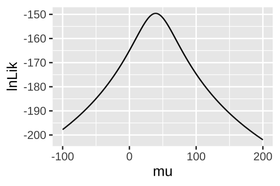

Figure 23.9: likelihood profile for proposed mean elevational shift in species examined by data from Chen et al. (2011)

maximium likelihood / confidence intervals / hypothesis testing

We can use the likelihood profile (Fig 23.9) to do standard things, like

make a best guess,
find confidence intervals,
test null hypotheses

First lets find our best guess – called the maximum likelihood estimator (MLE)

MLE <- lnLik_uphill %>%
  filter(lnLik == max(lnLik))

MLE

## [38;5;246m# A tibble: 1 x 2[39m
##      mu lnLik
##   [3m[38;5;246m<dbl>[39m[23m [3m[38;5;246m<dbl>[39m[23m
## [38;5;250m1[39m  39.3 -[31m150[39m[31m.[39m

Reassuringly, this MLE matches the simple calculation of the mean mean(observations) = 39.33.

Uncertainty We need one more trick to use the likelihood profile to estimate uncertainty

log likelihoods are roughly $\chi^2$ distributed with degrees of freedom equal to the number of parameters we’re inferring (here, just one – corresponding to the mean). So for 95% confidence intervals are everything within qchisq(p = .95, df =1) /2 = 1.92 log likelihood units of the MLE

CI <- lnLik_uphill %>%
  mutate(dist_from_MLE =  max(lnLik) - lnLik) %>%
  filter(dist_from_MLE < qchisq(p = .95, df =1) /2) %>%
  summarise(lower_95CI = min(mu),
            upper_95CI = max(mu))

CI

## [38;5;246m# A tibble: 1 x 2[39m
##   lower_95CI upper_95CI
##        [3m[38;5;246m<dbl>[39m[23m      [3m[38;5;246m<dbl>[39m[23m
## [38;5;250m1[39m       28.4       50.3

Hypothesis testing by the likelihood ratio test

We can find a p-value and test the null hypothesis by comparing the likelihood of our MLE ($log\mathcal{L}(MLE|D)$) to the likelihood of the null model ($log\mathcal{L}(H_0|D)$). We call this a likelihood ratio test, because we divide the likelihood of the MLE by the likelihood of the null – but we’re doing this in logs, so we subtract rather than divide.

$log\mathcal{L}(MLE|D)$ = Sum the log-likelihood of each observation under the MLE = pull(MLE, lnLik) = -149.594.
$log\mathcal{L}(H_0|D)$ = Sum the log-likelihood of each observation under the null = lnLik_uphill%>% filter(mu == 0 ) %>% pull(lnLik) = -164.989.

We then calculate $D$ which is simply two times this difference in lof likelihoods, and calcualte a p-value with it by noting that $D$ is $\chi^2$ distributed with degrees of freedom equal to the number of parameters we’re inferring (here, just one – corresponding to the mean).

D      <- 2 *  (pull(MLE, lnLik) -   lnLik_uphill%>% filter(mu == 0 ) %>% pull(lnLik)  )
p_val  <- pchisq(q = D, df = 1, lower.tail = FALSE)
tibble(D = D, p_val = p_val)

## [38;5;246m# A tibble: 1 x 2[39m
##       D        p_val
##   [3m[38;5;246m<dbl>[39m[23m        [3m[38;5;246m<dbl>[39m[23m
## [38;5;250m1[39m  30.8 0.000[4m0[24m[4m0[24m[4m0[24m028[4m7[24m

Bayesian inference

We often can are about how probable our model is given the data, not the opposite. We can use likelihoods to solve this!!! Remember Bayes’ theorem: $(Model|Data) = \frac{P(Data|Model) \times P(Model)}{P(Data)}$. Taking this apart

$(Model|Data)$ is called the posterior probability – the probability of our model after we know the data.
$P(Data|Model) = \mathcal{L}(Model|Data)$. This is the likelihood we just calculated.
$P(Model)$ is called the prior probability. This is the probability our model is true before we have data. We almost never know this, so we make something up that sounds reasonable…
$P(Data)$. The probability of our data, called the evidence. We find this through the law of total probability.

Today, we’ll arbitrarily pick a prior probability. This is a bad thing to do – out Bayesian inferences are only meaningful to the extent that a meaningfully interpret the posterior, and this relies on a reasonable prior. But we’re doing it as an example: – say our prior is that this is normally distributed around 0 with a standard deviation of 30.

bayes_uphill <- lnLik_uphill %>%
  mutate(lik   = exp(lnLik),
         prior = dnorm(x = mu, mean = 0, sd = 30) / sum(dnorm(x = mu, mean = 0, sd = 30) ),
         evidence  = sum(lik * prior),
         posterior =  (lik *  prior) / evidence)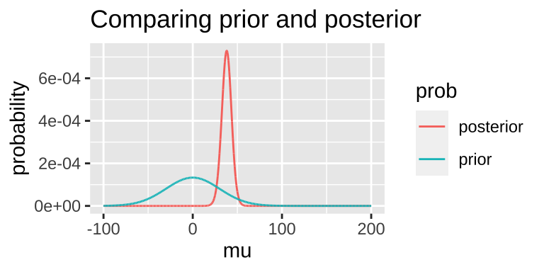

We can grab interesting thing from the posterior distribution.

For example we can find the maximum a posteriori (MAP) estimate as

bayes_uphill %>%
  filter(posterior == max(posterior))

## [38;5;246m# A tibble: 1 x 6[39m
##      mu lnLik      lik     prior evidence posterior
##   [3m[38;5;246m<dbl>[39m[23m [3m[38;5;246m<dbl>[39m[23m    [3m[38;5;246m<dbl>[39m[23m     [3m[38;5;246m<dbl>[39m[23m    [3m[38;5;246m<dbl>[39m[23m     [3m[38;5;246m<dbl>[39m[23m
## [38;5;250m1[39m  38.1 -[31m150[39m[31m.[39m 1.05[38;5;246me[39m[31m-65[39m 0.000[4m0[24m[4m5[24m[4m9[24m4 8.55[38;5;246me[39m[31m-67[39m  0.000[4m7[24m[4m2[24m[4m9[24m

Note that this MAP estimate does not equal our MLE as it is pulled away from it by our prior.

We can grab the 95% credible interval. Unlike the 95% confidence intervals, the 95% credible interval has a 95% chance of containing the true parameter (if our prior is correct).

bayes_uphill %>%
  mutate(cumProb = cumsum(posterior)) %>%
  filter(cumProb > 0.025 & cumProb < 0.975)%>%
  summarise(lower_95cred = min(mu),
            upper_95cred = max(mu))

## [38;5;246m# A tibble: 1 x 2[39m
##   lower_95cred upper_95cred
##          [3m[38;5;246m<dbl>[39m[23m        [3m[38;5;246m<dbl>[39m[23m
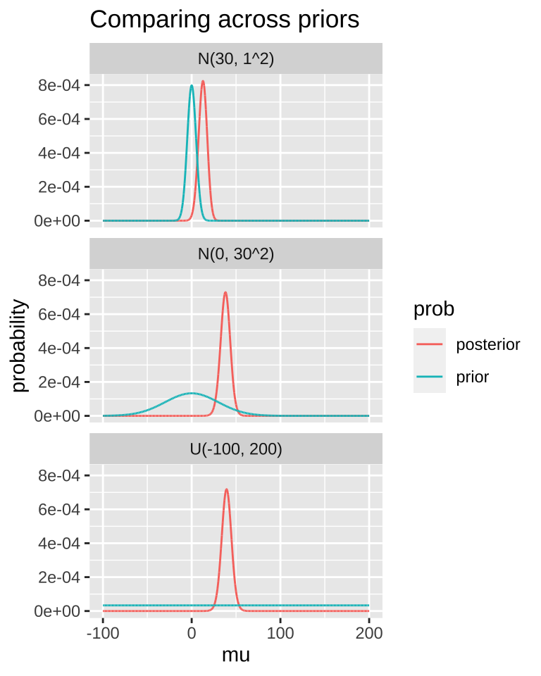
## [38;5;250m1[39m         26.8         48.9

Prior sensitivity

In a good world our priors are well calibrated.
In a better world, the evidence in the data is so strong, that our priors don’t matter.

A good thing to do is to compare our posterior distributions across different prior models. The plot below shows that if our prior is very tight, we have trouble moving the posterior away from it. Another way to say this, is that if your prior believe is strong, it would take loads of evidence to gr you to change it.

MCMC / STAN / brms

With more complex models, we usually can’t use the math above to solve Bayesian problems. Rather we use computer ticks – most notably the Markov Chain Monte Carlo MCMC to approximate the posterior distribution.

The programming here can be tedious so there are many programs – notable WINBUGS, JAGS and STAN – that make the computation easier. But even those can be a lot of work. Here I use the R package brms, which runs stan for us, to do an MCMC and do Bayesian stats. I suggest looking into this if you want to get stared, and learning STAN for more serious analyses

library(brms)
change.fit <- brm(elevationalRangeShift ~ 1, 
    data   = range_shift,
    family = gaussian(),
    prior  = set_prior("normal(0, 30)", 
                      class = "Intercept"),
    chains = 4,
    iter   = 5000)

change.fit$fit

## [38;5;246m# A tibble: 3 x 11[39m
##   term          mean se_mean    sd `2.5%`  `25%`  `50%`  `75%` `97.5%` n_eff  Rhat
##   [3m[38;5;246m<chr>[39m[23m        [3m[38;5;246m<dbl>[39m[23m   [3m[38;5;246m<dbl>[39m[23m [3m[38;5;246m<dbl>[39m[23m  [3m[38;5;246m<dbl>[39m[23m  [3m[38;5;246m<dbl>[39m[23m  [3m[38;5;246m<dbl>[39m[23m  [3m[38;5;246m<dbl>[39m[23m   [3m[38;5;246m<dbl>[39m[23m [3m[38;5;246m<dbl>[39m[23m [3m[38;5;246m<dbl>[39m[23m
## [38;5;250m1[39m b_Intercept   37.8    0.06  5.69   26.6   34.1   37.9   41.6    48.8  [4m7[24m863     1
## [38;5;250m2[39m sigma         31.7    0.05  4.25   24.8   28.7   31.2   34.2    41.3  [4m6[24m444     1
## [38;5;250m3[39m lp__        -[31m157[39m[31m.[39m     0.02  1.04 -[31m159[39m[31m.[39m  -[31m157[39m[31m.[39m  -[31m156[39m[31m.[39m  -[31m156[39m[31m.[39m   -[31m156[39m[31m.[39m   [4m4[24m340     1

23.9 Showing the t is like the z with unknown sd

n_reps      <- 5000
sample_size <- 10
mu_0        <- 50
pop_sd      <- 20

bind_rows(tibble(vals = rnorm(n = n_reps * sample_size, mean = mu_0, sd = pop_sd),
                 replicate = rep(1:n_reps, each = sample_size)) %>%
            group_by(replicate)%>%
            summarise(t = (mean(vals) - mu_0) / (sd(vals) /  sqrt(n())) ) %>%
            mutate(simulation = "normal n = 10"),
          tibble(t = rt(n = n_reps, df = 9),
                 simulation = "t. df = 9")) %>%
  ggplot(aes(x = t, fill = simulation))+
  geom_density(alpha = .2)+ theme(legend.position = "bottom")+
  labs(title = "Showing tha the t distribution works",
       subtitle = "Comparing rt(n = n_reps, df = 9) to the means of "
        )

## `summarise()` ungrouping output (override with `.groups` argument)

References

Chen, I-Ching, Jane K. Hill, Ralf Ohlemüller, David B. Roy, and Chris D. Thomas. 2011. “Rapid Range Shifts of Species Associated with High Levels of Climate Warming.” Science 333 (6045): 1024–26. https://doi.org/10.1126/science.1206432.

Rutte, Michael, Claudia AND Taborsky. 2007. “Generalized Reciprocity in Rats.” PLOS Biology 5 (7): 1–5. https://doi.org/10.1371/journal.pbio.0050196.

Whitlock, Michael C, and Dolph Schluter. 2020. The Analysis of Biological Data. Third Edition.