Chapter 39 Mixed models
Motivating scenario: We want to estimate account forthe variability among groups when making inference.
39.1 Review
39.1.1 Linear models
Remember, linear models predict Y as a deviation from some constant, a, as a function of a bunch of stuff.
\[\widehat{Y_i} = a + b_1 \times y_{1,i} + b_2 \times y_{2,i} + \dots\] Among the major assumptions of linear models is the independence of residuals, conditional on predictors. But in the real world, this assumption is often violated.
39.2 Multilevel (aka heirarchical) models
Of course, we can overcome this assumption of independence by modelling the dependence structure of the data. For example, if results of student’s tests are nondependent because they are in a class in a school we can put school and class into our model.
When we aren’t particularly interested in school or class themselves, these are called nuisance parameters.
When school (or class, or whatever “cluster” we’re concerned with) is chosen at random we can model it as a random effect. If not, we can use various other models, including generalized least squares (GLS), which we are not covering right now, but which have similar motivations.
39.3 Mixed effect models
How do we test for some fixed effect, like if type of math instruction increases math scores, in the presence of this nonindependence (like students in the same class learn from the same teacher etc…)?
In a mixed effect model, we model both fixed and random effects!!!!
39.3.1 Random Intercepts
With a “random intercept” each cluster gets its own intercept, which it drawn from some distribution. This on its own is much like the example in Chapter 38.
If we assume a random intercept only, we assume that each cluster draws an intercept from some distribution, but that clusters have the same slope (save what is specified in the fixed effect).
39.3.2 Random Slopes
With a “random slope” each cluster gets its own slope, which it drawn from some distribution.
If we assume a random slope only, we assume that each cluster draws a slope from some distribution, but that cluster have the same intercepts (save what is specified in the fixed effect).
39.3.3 Random Slopes and Random Intercepts
We can, in theory model both random slopes and random intercepts. But sometimes these are hard to estimate together, so be careful.
39.3.4 Visualizing Random Intercepts and Random Slopes
I find it pretty hard to explain random slopes and intercepts in words, but that pictures really help!
Read and scroll through the example below (from http://mfviz.com/hierarchical-models/), as it is the best description I’ve come across.
39.4 Mixed model: Random intercept example
Selenium, is a bi-product of burning coal. Could Selenium bioaccumulate in fish, suchb that fish from lakes with more selenium have more selenium in them?
Lets look at data (download here) from 98 fish from nine lakes, with 1 to 34 fish per lake.
39.4.1 Ignoring nonindependence is inapprorpiate
What if we just ignored lake and assumed each fish was independent???
selenium     <- read_csv("https://drive.google.com/uc?export=download&id=1UAkdZYLJPWRuFrq9Dc4StxfHCGW_43Ye")
selenium_lm1 <- lm(Log_fish_Se ~  Log_Water_Se, data = selenium)

summary(selenium_lm1)
##
## Call:
## lm(formula = Log_fish_Se ~ Log_Water_Se, data = selenium)
##
## Residuals:
## Min 1Q Median 3Q Max
## -0.7569 -0.3108 -0.1789 0.4301 0.8180
##
## Coefficients:
## Estimate Std. Error t value Pr(>|t|)
## (Intercept) 1.16351 0.06387 18.216 < 2e-16 ***
## Log_Water_Se 0.26483 0.05858 4.521 2.08e-05 ***
## ---
## Signif. codes: 0 '***' 0.001 '**' 0.01 '*' 0.05 '.' 0.1 ' ' 1
##
## Residual standard error: 0.4305 on 81 degrees of freedom
## Multiple R-squared: 0.2015, Adjusted R-squared: 0.1916
## F-statistic: 20.44 on 1 and 81 DF, p-value: 2.081e-05anova(selenium_lm1)## Analysis of Variance Table
##
## Response: Log_fish_Se
## Df Sum Sq Mean Sq F value Pr(>F)
## Log_Water_Se 1 3.787 3.7870 20.436 2.081e-05 ***
## Residuals 81 15.010 0.1853
## ---
## Signif. codes: 0 '***' 0.001 '**' 0.01 '*' 0.05 '.' 0.1 ' ' 1ggplot(selenium, aes(x = Log_Water_Se, y = Log_fish_Se, label = Lake)) +
geom_point(aes(color = Lake), alpha = .5, size = 3) +
geom_smooth(method = "lm")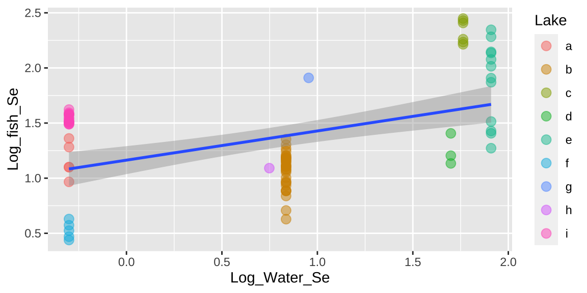
That would be a big mistake – as each fish is not independent. There could be something else about the lake associated with levels of Selenium in fish that is not in our model. This seems likely, as we see below, that residuals differ substantially by lake.
bind_cols( selenium ,
           augment(selenium_lm1)  %>%    dplyr::select(.resid))%>%
  ggplot(aes(x = Lake, y = .resid, color = Lake)) +
  geom_jitter(width = .2, size = 3, alpha =.6, show.legend = FALSE)+
  geom_hline(yintercept = 0, color = "red")+
  stat_summary(data = . %>% group_by(Lake) %>% mutate(n = n()) %>% dplyr::filter(n>1), color = "black")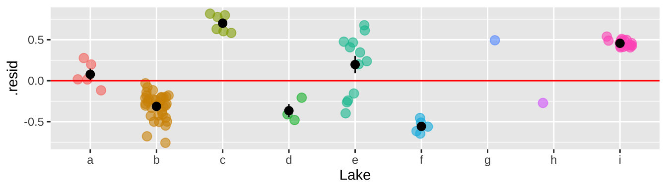
So why is this so bad? It’s because we keep pretending each fish is independent when it is not. So, our certainty is WAY bigger than it deserves to be. This means that our p-value is WAY smaller than it deserves to be.
39.4.2 We can’t model lake as a fixed effect
And even if we could it would be wrong.
Putting lake into our model as a fixed effect would essentially take the average of Fish Selenium content for each lake. Since each lake has only one Selenium content, we then have nothing to model.
lm(Log_fish_Se ~ Lake + Log_Water_Se, data = selenium) ##
## Call:
## lm(formula = Log_fish_Se ~ Lake + Log_Water_Se, data = selenium)
##
## Coefficients:
## (Intercept) Lakeb Lakec Laked Lakee Lakef Lakeg
## 1.16191 -0.08949 1.17069 0.08629 0.70488 -0.63493 0.74802
## Lakeh Lakei Log_Water_Se
## -0.07097 0.37860 NABut even when this is not the case, this is not the appropriate modelling strategy.
39.4.3 Taking averages is a less wrong thing
What if we just took the average selenium content over all fish for every lake, and then did our stats?
selenium_avg <- selenium %>%
  group_by(Lake, Log_Water_Se) %>%
  summarise(mean_log_fish_Se = mean(Log_fish_Se), n = n())

selenium_lm2 <- lm(mean_log_fish_Se ~  Log_Water_Se, data = selenium_avg)
summary(selenium_lm2)
##
## Call:
## lm(formula = mean_log_fish_Se ~ Log_Water_Se, data = selenium_avg)
##
## Residuals:
## Min 1Q Median 3Q Max
## -0.50657 -0.36536 0.03456 0.42871 0.55425
##
## Coefficients:
## Estimate Std. Error t value Pr(>|t|)
## (Intercept) 1.1307 0.2094 5.399 0.00101 **
## Log_Water_Se 0.3673 0.1807 2.032 0.08161 .
## ---
## Signif. codes: 0 '***' 0.001 '**' 0.01 '*' 0.05 '.' 0.1 ' ' 1
##
## Residual standard error: 0.4653 on 7 degrees of freedom
## Multiple R-squared: 0.3711, Adjusted R-squared: 0.2813
## F-statistic: 4.131 on 1 and 7 DF, p-value: 0.08161anova(selenium_lm2)## Analysis of Variance Table
##
## Response: mean_log_fish_Se
## Df Sum Sq Mean Sq F value Pr(>F)
## Log_Water_Se 1 0.89428 0.89428 4.131 0.08161 .
## Residuals 7 1.51536 0.21648
## ---
## Signif. codes: 0 '***' 0.001 '**' 0.01 '*' 0.05 '.' 0.1 ' ' 1ggplot(selenium_avg, aes(x = Log_Water_Se, y = mean_log_fish_Se, label = Lake)) +
geom_point(aes(size = n)) +
geom_text_repel(aes(color = Lake), show.legend = FALSE) +
geom_smooth(method = "lm",se = FALSE)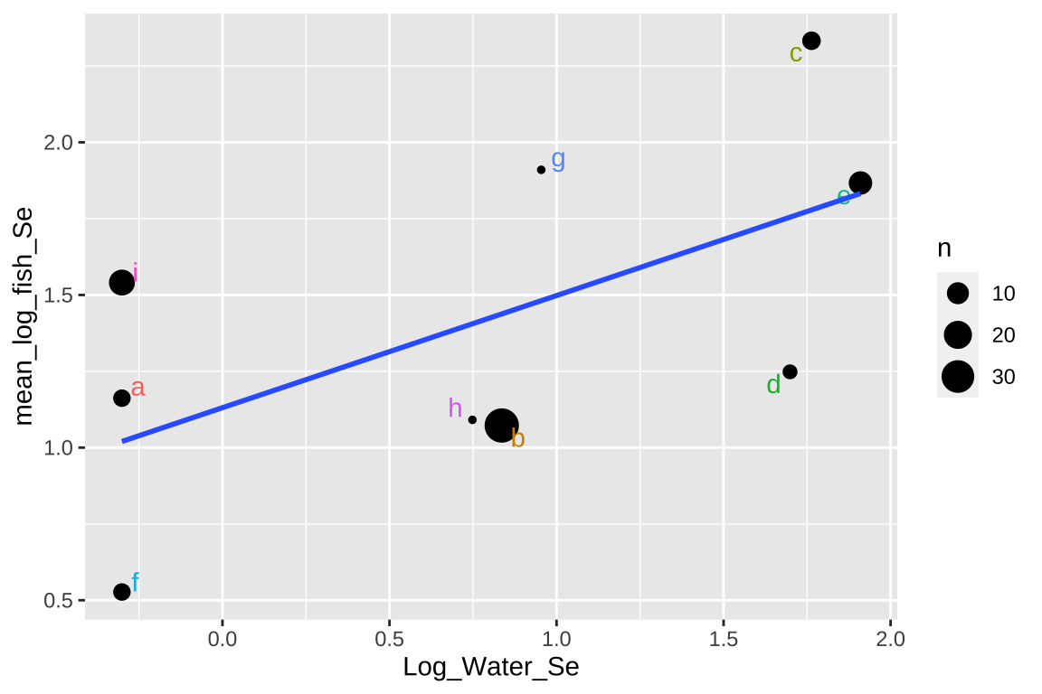
This approach isn’t too bad, but there are some shortcomings –
- It takes all means as equally informative, even though some come from large and others from large samples.
- It ignores variability within each lake,
- It surrenders so much of our hard-won data.
39.4.4 Accounting for Lake as a Random Effect is our best option
Rather, we can model Lake as a random effect – this allows us to model the non-independence of observations within a Lake, while using all of the data.
selenium_lme <- lmer(Log_fish_Se ~   (1|Lake) + Log_Water_Se , data = selenium)
summary(selenium_lme)
## Linear mixed model fit by REML. t-tests use Satterthwaite's method ['lmerModLmerTest']
## Formula: Log_fish_Se ~ (1 | Lake) + Log_Water_Se
## Data: selenium
##
## REML criterion at convergence: -8.8
##
## Scaled residuals:
## Min 1Q Median 3Q Max
## -3.15542 -0.37400 0.04239 0.54953 2.54730
##
## Random effects:
## Groups Name Variance Std.Dev.
## Lake (Intercept) 0.20747 0.4555
## Residual 0.03548 0.1884
## Number of obs: 83, groups: Lake, 9
##
## Fixed effects:
## Estimate Std. Error df t value Pr(>|t|)
## (Intercept) 1.1322 0.2089 6.8420 5.419 0.00107 **
## Log_Water_Se 0.3659 0.1794 6.7266 2.039 0.08249 .
## ---
## Signif. codes: 0 '***' 0.001 '**' 0.01 '*' 0.05 '.' 0.1 ' ' 1
##
## Correlation of Fixed Effects:
## (Intr)
## Log_Water_S -0.666Thus we fail to reject the null, and conclude that there is not sufficient evidence to support the idea that more selenium in lakes is associated with more selenium in fish.
39.4.4.1 Extracting estimates and uncertainty
Alhough we do have model estimates, degrees of freedom and standard deviations above, if ca still be hard to consider and commuincate uncertainty. The ggpredict function in the ggeffects package can help!
library(ggeffects)
gg_color_hue <- function(n) {hues = seq(15, 375, length = n + 1); hcl(h = hues, l = 65, c = 100)[1:n]}

selenium_predictions <- ggpredict(selenium_lme, terms = "Log_Water_Se")
selenium_predictions
## # Predicted values of Log_fish_Se
## # x = Log_Water_Se
##
## x | Predicted | 95% CI
## --------------------------------
## -0.30 | 1.02 | [0.54, 1.51]
## 0.75 | 1.41 | [1.10, 1.71]
## 0.84 | 1.44 | [1.13, 1.74]
## 0.95 | 1.48 | [1.17, 1.79]
## 1.70 | 1.75 | [1.31, 2.20]
## 1.76 | 1.78 | [1.31, 2.24]
## 1.91 | 1.83 | [1.33, 2.33]
##
## Adjusted for:
## * Lake = 0 (population-level)plot(selenium_predictions)+
geom_point(data = selenium, aes(x = Log_Water_Se , y= Log_fish_Se, color = Lake), alpha = .4, size = 3)+
scale_color_manual(values = gg_color_hue(9))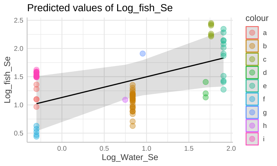
39.4.4.2 Evaluating assumptions
We can now see that by modeling Lake as a random effect, the residuals are now independent.
bind_cols( selenium ,
           broom.mixed::augment(selenium_lme)  %>%    dplyr::select(.resid))%>%
  ggplot(aes(x = Lake, y = .resid, color = Lake)) +
  geom_jitter(width = .2, size = 3, alpha =.6, show.legend = FALSE)+
  geom_hline(yintercept = 0, color = "red")+
  stat_summary(data = . %>% group_by(Lake) %>% mutate(n = n()) %>% dplyr::filter(n>1),color = "black")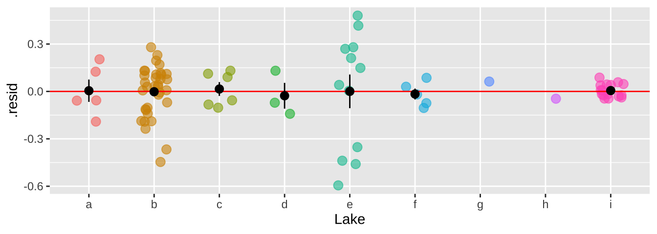
Major assumptions of linear mixed effect models are
- Data are collected without bias
- Clausters are random
- Data cna be modelled as a linear function of predictors
- Variance of the reiduals is indpednet of predicted values,
- Residuals are normally distributed,
Let’s look into the last two for these data. Because we hate autoplot, and it can’t handle random effects outplut, let’s make out own diangnostic plots.
selenium_qq <- broom.mixed::augment(selenium_lme) %>%
  ggplot(aes(sample = .resid))+
  geom_qq()+
  geom_qq_line()

selenium_std_resid  <- broom.mixed::augment(selenium_lme) %>%
  mutate(sqrt_abs_std_resid = sqrt(abs(.resid / sd(.resid)) )) %>%
  ggplot(aes(x = .fitted, y = sqrt_abs_std_resid)) +
  geom_point()

plot_grid(selenium_qq, selenium_std_resid, ncol = 2)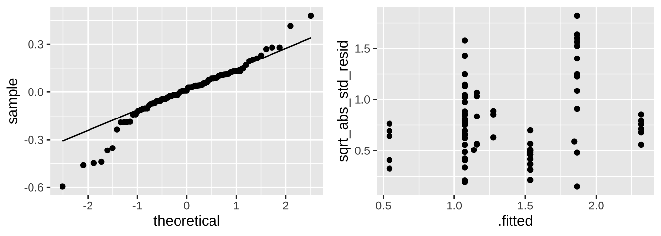
These don’t look great tbh. We would need to think harder if we where doing a legitimate analysis.
39.5 Example II: Loblolly Pine Growth
Let’s try to model the growth rate of loblolly pines!
First I looked at the data (a), and thought a square root transfrom would be a better linear model (b), expecially if I began my model after threee years of growth (c).
Loblolly <- mutate(Loblolly, Seed = as.character(Seed))
a <- ggplot(Loblolly, aes(x = age, y = height, group = Seed, color = Seed))+ geom_line()
b <- ggplot(Loblolly, aes(x = sqrt(age), y = height, group = Seed, color = Seed))+ geom_line()
c <- ggplot(Loblolly %>% filter(age > 3), aes(x = sqrt(age), y = height, group = Seed, color = Seed))+ geom_line()
top  <- plot_grid(a+theme(legend.position = "none"),
                  b+theme(legend.position = "none"),
                  c+theme(legend.position = "none") ,
                  labels = c("a","b","c"), ncol = 3)
legend<- get_legend(a+ guides(color = guide_legend(nrow=2)) + theme(legend.position = "bottom", legend.direction = "horizontal") )
plot_grid(top, legend, ncol =1, rel_heights = c(8,2))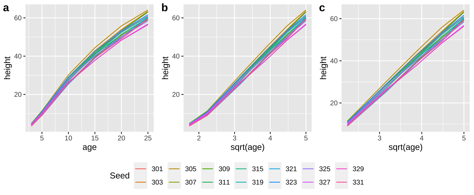
39.5.1 Random Slopes
loblolly_rand_slope <- lmer(height ~ age + (0+age|Seed), data = filter(Loblolly, age>3))
summary(loblolly_rand_slope)
## Linear mixed model fit by REML. t-tests use Satterthwaite's method ['lmerModLmerTest']
## Formula: height ~ age + (0 + age | Seed)
## Data: filter(Loblolly, age > 3)
##
## REML criterion at convergence: 348.6
##
## Scaled residuals:
## Min 1Q Median 3Q Max
## -1.6115 -0.9585 0.1945 0.7035 1.8126
##
## Random effects:
## Groups Name Variance Std.Dev.
## Seed age 0.005779 0.07602
## Residual 7.116593 2.66769
## Number of obs: 70, groups: Seed, 14
##
## Fixed effects:
## Estimate Std. Error df t value Pr(>|t|)
## (Intercept) 0.73121 0.74777 55.00001 0.978 0.332
## age 2.48390 0.04946 61.41943 50.222 <2e-16 ***
## ---
## Signif. codes: 0 '***' 0.001 '**' 0.01 '*' 0.05 '.' 0.1 ' ' 1
##
## Correlation of Fixed Effects:
## (Intr)
## age -0.825broom.mixed::augment(loblolly_rand_slope) %>% mutate(Seed = as.character(Seed)) %>%
ggplot(aes(x = age, y = .fitted, color = Seed)) +
geom_line() + theme(legend.position = "none")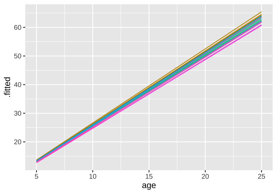
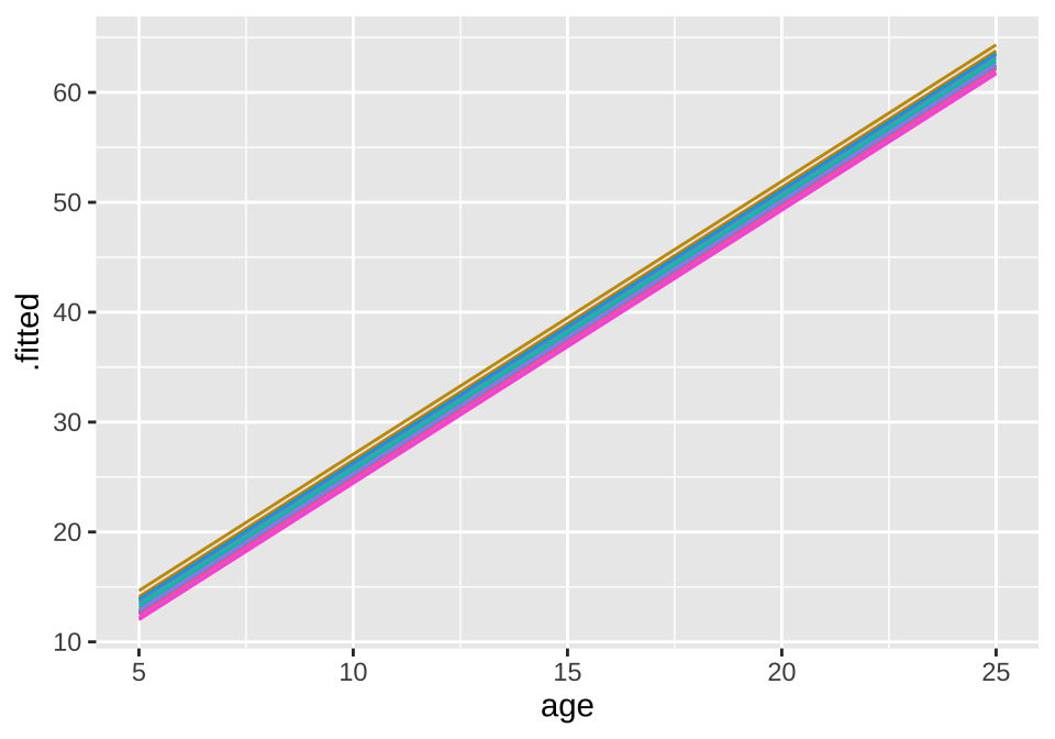
39.5.2 Random Intercepts
loblolly_rand_intercept <- lmer(height ~ age + (1|Seed), data = filter(Loblolly, age>3))
summary(loblolly_rand_intercept)
## Linear mixed model fit by REML. t-tests use Satterthwaite's method ['lmerModLmerTest']
## Formula: height ~ age + (1 | Seed)
## Data: filter(Loblolly, age > 3)
##
## REML criterion at convergence: 349.6
##
## Scaled residuals:
## Min 1Q Median 3Q Max
## -1.9391 -0.9836 0.2641 0.7693 1.8060
##
## Random effects:
## Groups Name Variance Std.Dev.
## Seed (Intercept) 1.318 1.148
## Residual 7.376 2.716
## Number of obs: 70, groups: Seed, 14
##
## Fixed effects:
## Estimate Std. Error df t value Pr(>|t|)
## (Intercept) 0.73121 0.82078 63.47415 0.891 0.376
## age 2.48390 0.04591 55.00000 54.109 <2e-16 ***
## ---
## Signif. codes: 0 '***' 0.001 '**' 0.01 '*' 0.05 '.' 0.1 ' ' 1
##
## Correlation of Fixed Effects:
## (Intr)
## age -0.839broom.mixed::augment(loblolly_rand_intercept) %>% mutate(Seed = as.character(Seed)) %>%
ggplot(aes(x = age, y = .fitted, color = Seed)) +
geom_line() + theme(legend.position = "none")