Chapter 25 Two samples from normal distributions
Motivating scenarios: We are interested to investigate the difference between the means of two samples.
Learning goals: By the end of this chapter you should be able to
- Know when and how to use a two-sample t-test.
- Recognize the difference between a paired and two-sample t-test.
- Recognize the difference between a paired and two-sample t-test.
- Work through the math underlying a two-sample t-test.
- Connect the two-sample t-test to a simple linear model.
- State the assumptions of a two-sample t-test, as a specific case of the general assumptions of a linear model.
- Know alternatives to a two sample t-test when data break assumptions
25.1 Review: What is a linear model?
A statistical model describes the predicted value of a response variable as a function of one or more explanatory variables. \(\hat{Y_i} = f(\text{explanatory variables}_i)\)
A linear model predicts the response variable by adding up all components of the model. \(\hat{Y_i} = a + b_1 y_{1,i} + b_2 y_{2,i} + \dots{}\).
25.1.1 Review: A two-sample t-test as a linear model
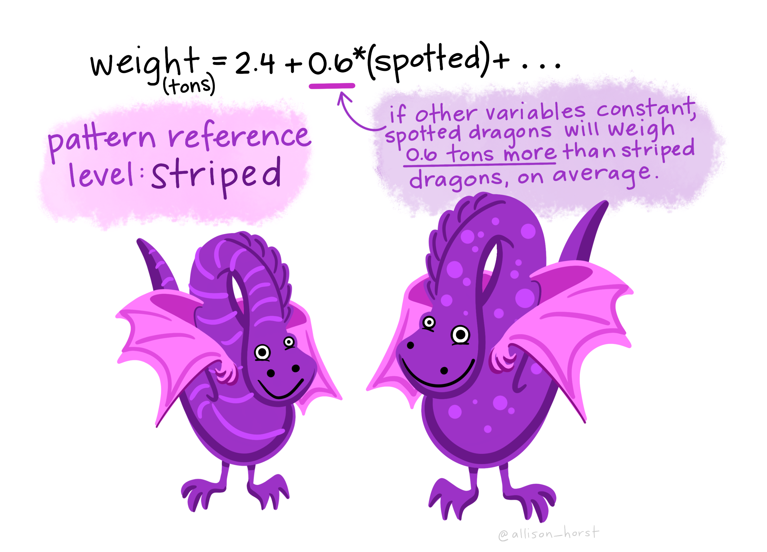
We often want to know the difference in means between two (unpaired) groups, and test the null hypothesis that these means are identical. For this linear model,
- \(a\) is the estimate mean for one group,
- \(b_1\) is the average difference between individuals in that and the other group.
- \(y_{1,i}\) is an “indicator variable” equaling zero for individuals in group 1 and one for individuals in the other group.
So, the equation \(\hat{Y_i} = a + Y_{1,i} \times b_1\) is
\[\begin{equation} \hat{Y_i}= \begin{cases} a + 0 \times b_1 & = a, &\text{if }\ i \text{ is in group 1}\\ a + 1 \times b_1 & = a +b_1, &\text{if }\ i\text{ is in group 2} \end{cases} \end{equation}\]
25.1.1.1 Previous Example: Lizard survival
Could long spikes protect horned lizards from being killed by the loggerhead shrike? The loggerhead shrike is a small predatory bird that skewers its victims on thorns or barbed wire. Young, Brodie, and Brodie (2004) compared horns from lizards that had been killed by shrikes to 154 live horned lizards. The data are plotted below.
lizards <- read_csv("https://whitlockschluter3e.zoology.ubc.ca/Data/chapter12/chap12e3HornedLizards.csv") %>% na.omit()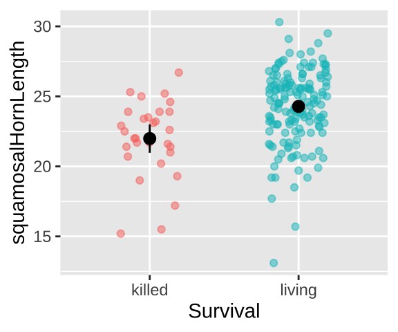
Living Lizard summary stats: From our sample of 154 living lizards, the mean horn length was 24.28, with a sample variance of 6.92.
Killed Lizard summary stats: From our sample of 30 killed lizards, the mean horn length was 22, with a sample variance of 7.34.
Summarizing the difference in Killed and Living lizards: So, surviving lizards have horns that are 2.29 longer than killed lizards.
Lizard survival as a linear model
From these values, we can describe the horn length of the \(i^{th}\) lizard as
\[\begin{equation} \begin{split} Y_i &= \hat{Y_i} +e_i \\ &= 22.0 + \text{living}_i \times 2.29 + e_i \end{split} \tag{25.1} \end{equation}\]
Where \(e_i\) is the residual difference between group mean and the value of individual, \(i\), and living is an indicator variable which equals one if living, and 0 if killed. This trick thinks of a lizard as a killed lizard, and then adds 2.29 mm to this length if the lizard survived.
lizard_lm <- lm(squamosalHornLength ~ Survival, data = lizards)
lizard_lm %>% tidy()
## [38;5;246m# A tibble: 2 x 5[39m
## term estimate std.error statistic p.value
## [3m[38;5;246m<chr>[39m[23m [3m[38;5;246m<dbl>[39m[23m [3m[38;5;246m<dbl>[39m[23m [3m[38;5;246m<dbl>[39m[23m [3m[38;5;246m<dbl>[39m[23m
## [38;5;250m1[39m (Intercept) 22.0 0.483 45.6 1.90[38;5;246me[39m[31m-101[39m
## [38;5;250m2[39m Survivalliving 2.29 0.528 4.35 2.27[38;5;246me[39m[31m- 5[39mR’s output describes this as
(Intercept)of 22.0 – the mean horn length of killed lizards, and
Survivallivinghow much longer, on average horn length is in surviving lizards.
Remember that the t value and p-value for the (Intercept) describe the difference between estimated horn length and zero, a silly null hypothesis, so we consider this estimate and our uncertainty around it, but ignore that \(t\) and p-value. The t value and p-value for the Survivalliving describe the difference between estimated horn length of surviving and dead lizards. The \(t\) value of 4.35 means that the observed 2.29 mm difference in horn length is four and a third standard errors (four and a third standard deviations of the sampling distribution) away from the expected difference of zero.
25.2 Calculations for a two sample t-test
So, where did these numbers, and more specifically the standard error come from? How do we describe our uncertainty in this difference in means? And how do we describe the effect size of this difference? To start to answer these questions we need to describe the within group variance in horn length.
25.2.1 The pooled variance
How do we think about this variance? I like to think of it as “how far on average do we expect the square of the difference between one random individual from each group to deviate from the average difference between groups.” A quantity that nearly captures this is the pooled variance, \(s_p^2\), which is the variance in each group weighted by the degrees of freedom in each group, \(df_1\) and \(df_2\) and divided by the total degrees of freedom, \(df_t = df_1+df_2\).
\[\begin{equation} \begin{split} s_p^2 &= \frac{df_1\times s_1^2+df_2\times s_2^2}{df_1+df_2} \end{split} \tag{25.2} \end{equation}\]
Calculating the pooled variance in the lizard example
Recall that we had 154 living lizards, with a sample variance in horn length of 6.92 and 30 killed lizards, with a sample variance in horn length of 7.34. So in this case, the pooled variance is
\[\begin{equation}
\begin{split}
s_p^2 &= \frac{df_1\times s_1^2+df_2\times s_2^2}{df_1+df_2}\\
&= \frac{df_\text{living}\times s_\text{living}^2+df_\text{killed}\times s_\text{killed}^2}{df_\text{living}+df_\text{killed}}\\
&= \frac{(154-1)\times 6.92 + (30-1)\times 7.34}{154 + 30 -2} \\
&= 6.99
\end{split}
\tag{25.3}
\end{equation}\]
We can do this math in R
# First we get the summaries
lizard_summaries <- lizards %>%
  group_by(Survival) %>%
  summarise(n         = n(),
            df        = n - 1,
            mean_horn = mean(squamosalHornLength),
            var_horn  = var(squamosalHornLength))

# Then we calculate the pooled variance
lizard_summaries %>%
  summarise(pooled_variance = sum(df * var_horn) / sum(df) )
## [38;5;246m# A tibble: 1 x 1[39m
## pooled_variance
## [3m[38;5;246m<dbl>[39m[23m
## [38;5;250m1[39m 6.99Effect size of the difference in Killed and Living lizards: Above we found that surviving lizards have horns that are 2.29 longer than killed lizards. But recall that our estimate of effect size, Cohen’s D, standardizes this difference by the standard deviation to give it more context. The math below shows that the average surviving lizard has a horn about 0.87 standard deviations larger than the average killed lizard. That’s pretty substantial.
\[\text{Cohen's d } = \frac{\text{distance from null}}{s} = \frac{24.28 - 21.99}{\sqrt{ 6.99}} = \frac{2.29}{\sqrt{ 2.64}} = 0.87\]
25.2.2 The standard error
So Cohen’s d showed a very large difference in horn lengths. But how does this difference compare to what we expect by sampling error?
We could, of course, get a sense of this sampling error by resampling from each group with replacement, and calculating the mean difference for each “bootstrapped” replicate to approximate a sampling distribution, and use this to calculate a standard error and confidence interval
living_lizards <- filter(lizards, Survival == "living")
dead_lizards <- filter(lizards, Survival == "killed")
full_join(
  rep_sample_n(living_lizards, size = nrow(living_lizards), replace = TRUE, reps = 100000) %>%
    summarise(mean_living_horn = mean(squamosalHornLength)),
  rep_sample_n(dead_lizards, size = nrow(dead_lizards), replace = TRUE, reps = 100000) %>%
    summarise(mean_dead_horn = mean(squamosalHornLength)),  by = "replicate") %>%
  mutate(boot_diff = mean_living_horn - mean_dead_horn) %>%
  summarise(se = sd(boot_diff),
            lower_CI = quantile(boot_diff, prob = 0.025),
            upper_CI = quantile(boot_diff, prob = 0.975))
## [38;5;246m# A tibble: 1 x 3[39m
## se lower_CI upper_CI
## [3m[38;5;246m<dbl>[39m[23m [3m[38;5;246m<dbl>[39m[23m [3m[38;5;246m<dbl>[39m[23m
## [38;5;250m1[39m 0.531 1.29 3.37Alternatively, we can use math tricks to estimate the standard error. Specifically, the standard error for the difference in means, \(SE_{\overline{x_1}-\overline{x_2}}\) equals \(SE_{\overline{x_1}-\overline{x_2}} = \sqrt{s_p^2 \Big(\frac{1}{n_1} + \frac{1}{n_2}\Big)}\), where \(s_p^2\) is the pooled variance from Equation (25.2). In this case, \(SE_{\overline{x_1}-\overline{x_2}} = \sqrt{6.99 \Big(\frac{1}{154} + \frac{1}{30}\Big)} 0.58\).
As in Chapter 23, we can use equation (23.1) – \((1-\alpha)\%\text{ CI } = \overline{x} \pm t_{\alpha/2} \times SE_x\) – to find the upper and lower confidence intervals.
Again, we can do these calculations in R. We see below that these mathematical answers are really close to the bootstrapped based estimates of uncertainty.
alpha <- 0.05
lizard_summaries %>%
  summarise(est_diff        = abs(diff(mean_horn)),
            pooled_variance = sum(df * var_horn) / sum(df),
            se              = sqrt(sum(pooled_variance/n)),
            crit_t_95       = qt(p = alpha/2, df = sum(df), lower.tail = FALSE),
            lower_95CI       = est_diff  - se * crit_t_95,
            upper_95CI       = est_diff  + se * crit_t_95)
## [38;5;246m# A tibble: 1 x 6[39m
## est_diff pooled_variance se crit_t_95 lower_95CI upper_95CI
## [3m[38;5;246m<dbl>[39m[23m [3m[38;5;246m<dbl>[39m[23m [3m[38;5;246m<dbl>[39m[23m [3m[38;5;246m<dbl>[39m[23m [3m[38;5;246m<dbl>[39m[23m [3m[38;5;246m<dbl>[39m[23m
## [38;5;250m1[39m 2.29 6.99 0.528 1.97 1.25 3.3425.2.3 Quantifying surprise
How surprised would we be to see such an extreme difference if we expected no difference at all? The p-value quantifies this surprise.
We can, of course estimate this by permutation
obs_diff <- lizard_summaries %>% summarise(diff(mean_horn)) %>% pull() %>% abs()

rep_sample_n(lizards, size =nrow(lizards),replace = FALSE, reps=500000) %>% # copyind
  mutate(Survival = sample(Survival))              %>%  # shuffling!
  group_by(replicate, Survival)                    %>%
  summarise(perm_mean = mean(squamosalHornLength)) %>% #mean of each group for each permuted replicate
  group_by(replicate)                              %>%
  summarise(perm_diff = abs(diff(perm_mean)))      %>%
  mutate(as_or_more = perm_diff >= obs_diff)       %>% # are the permutations as or more extreme
  summarise(p_val = mean(as_or_more))                  # what proportion are of permutations are as or more extreme?
## [38;5;246m# A tibble: 1 x 1[39m
## p_val
## [3m[38;5;246m<dbl>[39m[23m
## [38;5;250m1[39m 0.000[4m0[24m[4m3[24mWe find a very small p-value and reject the null hypothesis.
Alternatively, we could
- Calculate a t-value (as we did in Chapter 23).
- Compare the observed t to t’s sampling distribution with 182 degrees of freedom
- Find the area that exceeds our observed \(t\) on either tail of the distribution.
So, we first find our t-value as \(\frac{est - \mu_0}{se} = \frac{2.294-0}{0.5274} = 4.35\). We then compare it to its null sampling distribution. Figure 25.1 makes it clear that the p-value is very small – we need to zoom in on the null sampling distribution substantially to see anything as or more extreme
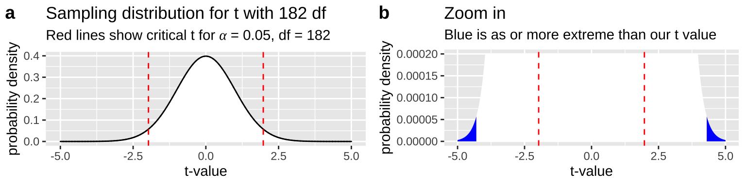
Figure 25.1: The null sampling distribution for t with 182 degrees of freedom. From a it is clear that our t is exceptional. Zooming in (b) we see very little of the sampling distribution is as or more extreme than our test stat of 4.35 (blue).
The exact p-value is 2 x pt(4.35, df = 182, lower.tail = FALSE) = 2.3^{-5}. We can calcualte this in R
lizard_summaries %>%
  summarise(est_diff        = abs(diff(mean_horn)),
            pooled_variance = sum(df * var_horn) / sum(df),
            se              = sqrt(sum(pooled_variance/n)),
            t               = est_diff / se,
            p               = 2 * pt(t, df = sum(df), lower.tail = FALSE))
## [38;5;246m# A tibble: 1 x 5[39m
## est_diff pooled_variance se t p
## [3m[38;5;246m<dbl>[39m[23m [3m[38;5;246m<dbl>[39m[23m [3m[38;5;246m<dbl>[39m[23m [3m[38;5;246m<dbl>[39m[23m [3m[38;5;246m<dbl>[39m[23m
## [38;5;250m1[39m 2.29 6.99 0.528 4.35 0.000[4m0[24m[4m2[24m[4m2[24m725.3 A two sample t-test in R
There are a few ways to conduct a two sample t-test in R –
25.3.1 With the t.test() function
- First, we could use the
t.test()function.
t.test(squamosalHornLength ~ Survival, data = lizards, var.equal = TRUE)##
## Two Sample t-test
##
## data: squamosalHornLength by Survival
## t = -4.3494, df = 182, p-value = 2.27e-05
## alternative hypothesis: true difference in means is not equal to 0
## 95 percent confidence interval:
## -3.335402 -1.253602
## sample estimates:
## mean in group killed mean in group living
## 21.98667 24.28117Piping this outpot to tidy makes it more compact
library(broom)
t.test(squamosalHornLength ~ Survival, data = lizards, var.equal = TRUE) %>%
  tidy()
## [38;5;246m# A tibble: 1 x 10[39m
## estimate estimate1 estimate2 statistic p.value parameter conf.low conf.high method alternative
## [3m[38;5;246m<dbl>[39m[23m [3m[38;5;246m<dbl>[39m[23m [3m[38;5;246m<dbl>[39m[23m [3m[38;5;246m<dbl>[39m[23m [3m[38;5;246m<dbl>[39m[23m [3m[38;5;246m<dbl>[39m[23m [3m[38;5;246m<dbl>[39m[23m [3m[38;5;246m<dbl>[39m[23m [3m[38;5;246m<chr>[39m[23m [3m[38;5;246m<chr>[39m[23m
## [38;5;250m1[39m -[31m2[39m[31m.[39m[31m29[39m 22.0 24.3 -[31m4[39m[31m.[39m[31m35[39m 2.27[38;5;246me[39m[31m-5[39m 182 -[31m3[39m[31m.[39m[31m34[39m -[31m1[39m[31m.[39m[31m25[39m Two Sa… two.sidedReassuringly, R’s output matches our calculations (but it swaps group 1 and 2, so watch out for that)
25.3.2 With the lm() function
We have already seen that we can consider this as a linear mode lizard_lm <- lm(squamosalHornLength ~ Survival, data = lizards). Looking at this output, se see that the p and t-values are the same as those we got for our t-test, so that’s good!
tidy(lizard_lm)## [38;5;246m# A tibble: 2 x 5[39m
## term estimate std.error statistic p.value
## [3m[38;5;246m<chr>[39m[23m [3m[38;5;246m<dbl>[39m[23m [3m[38;5;246m<dbl>[39m[23m [3m[38;5;246m<dbl>[39m[23m [3m[38;5;246m<dbl>[39m[23m
## [38;5;250m1[39m (Intercept) 22.0 0.483 45.6 1.90[38;5;246me[39m[31m-101[39m
## [38;5;250m2[39m Survivalliving 2.29 0.528 4.35 2.27[38;5;246me[39m[31m- 5[39m25.4 Assumptions
Before we worry about assumptions, let’s take a minute to think about assumptions in statistics. What is an assumption? What happens when we break one?
An assumption is basically a statement we make for mathematical convenience. We do this to make stats tractable (otherwise we’d either be doing different math for each data set or bootstrapping and permuting only).
- If data meet assumptions, we can be confident that our statistics will work as intended.
- If data break assumptions, the stats could still work. Or they could not. There are no guarantees, and no refunds.
But often breaking assumptions does not break a test. In fact, many statistical tests are remarkably robust to violations of their assumptions (but some are not).
How can we know if breaking an assumption will break our stats or if it’s safe?
- The easiest way is to ask someone who knows.
- The best way is to simulate.
We will simulate soon to show you what I mean, but for now, trust me, I know.
25.4.1 Assumptions of linear models
Remember that all linear models assume: Linearity, Homoscedasticity, Independence, Normality (of residual values, or more specifically, of their sampling distribution), and that Data are collected without bias.
25.4.2 Assumptions of the two-sample t-test
We can ignore the linearity assumption for a two sample t-test.
While we can never ignore bias or non-independence, we usually need more details of study design to get at them, so let’s focus on homoscedasticity and normality.
25.4.3 The two sample t-test assumes equal variance among groups
This makes sense as we used a “pooled variance” in the two sample t-test – that is, in the math we assume that both groups have equal variance equal to the pooled variance.
- Homoscedasticity means that the variance of residuals is independent of the predicted value. In this case we only make two predictions – one per group – so this essentially means that we assume equal variance in each group. Let’s evaluate this prediction by making a histogram of the residuals – remembering that the
augment()function in thebroompackage can find residuals for us.
augment(lizard_lm) %>%
  ggplot(aes(x = .resid, fill = Survival))+
  geom_histogram(show.legend = FALSE)    +
  facet_wrap(~Survival, scales = "free_y", ncol = 1)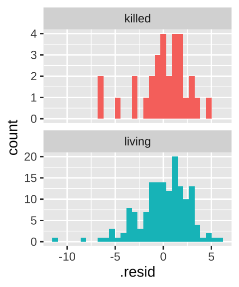
This similar distribution of residuals lines up with our calculations of a variance of 6.92, and 7.34 in living and killed lizards respectively. That’s pretty similar.
How similar must variances be to make a two-sample t-test ok? We’ll explore this soon, when we’ll see that the t-test is robust to violations of this assumption. In fact, as a rule of thumb, if variance in one group is less than five times the variance in the other group, we’re usually ok.
25.4.4 The two-sample t-test assumes normally disributed residuals
Note this means we assume the differences from group means are normally distributed, not that the raw data are.
As we saw for a one sample t-test in Chapter 23, the two sample t-test is quite robust to this assumption, as we are actually assuming a normal sampling distribution of residuals, rather than a normal distribution of residuals.
We could evaluate this assumption with the autoplot() function in the ggfortify package. But let’s just do this our self by making a qqplot
augment(lizard_lm) %>%
  ggplot(aes(sample = .resid))+
  geom_qq()+
  geom_qq_line()+
  labs(title = "qq plot of residuals from lizrd data")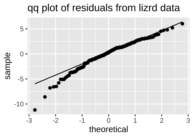
The data are obviously not normal, as the small values are too small (below the qq line). But the sample size is pretty big, so I would feel comfortable assuming normality here.
25.5 Alternatives to a two sample t-test
So, what to do if we break assumptions.
- We could ignore the violation, especially if it is minor and we believe the test is robust.
- We could transform the data, as described in Chapter 22.
- Or we could find a better test.
Let’s start at the bottom of the list – what are alternatives to the two-sample t-test?
25.5.1 Permutation / bootstrapping
We saw above that we can bootstrap (i.e. resample with replacement) to estimate uncertainty in the estimate of the mean difference, and we can permute (i.e. shuffle labels) to generate a null sampling distribution for hypothesis testing.
These approaches make nearly no assumptions and most always work, but generally require modest sample sizes of at least fifteen in each group or so, such that resampling from them with replacement generates enough combinations to reasonably approximate the sampling distribution from a population.
25.5.2 Welch’s t-test when variances differ by group
If the variances differ by group, we could do a Welch’s t-test, which does not assume equal variance. Here we use a different equation to calculate the t value and degrees of freedom 25.8, which you need never know.
Do know
- That you can use Welch’s t-test when variance differs by group.
- You can easily conduct a Welch’s t-test in R with the
t.test()function by settingvar.equalequal toFALSE. In fact, this is the default behavior of tis function in R.
t.test(squamosalHornLength ~ Survival, data = lizards, var.equal = FALSE)##
## Welch Two Sample t-test
##
## data: squamosalHornLength by Survival
## t = -4.2634, df = 40.372, p-value = 0.0001178
## alternative hypothesis: true difference in means is not equal to 0
## 95 percent confidence interval:
## -3.381912 -1.207092
## sample estimates:
## mean in group killed mean in group living
## 21.98667 24.28117All interpretations of results from the Welch’s t-test are the same as a interpretations of stats from a two sample t-test
- The t value is still the distance, in standard errors, between the observed difference in sample means and the null (0) away from one.
- The p-value is still the proportion of draws from the null that will be as or more extreme than our test statistic.
The only difference is that now the sampling distribution uses the variance from each group, rather than combining the variance into its average, “pooled variance.”
25.5.3 Mann-Whitney U and Wilcoxon rank sum tests
If residuals are not normal, we would usually do a permutation test nowadays. Historically, however, people used “rank based” “non parametric” tests when data weren’t normal. Here we
- Convert all data from their actual values to their “rank” (e.g. first, second, third, etc..) in the data set.
- Turn the distribution of ranks into a test statistic.
- Find a sampling distribution for ranks under a null model.
- Calculate a p-value, and reject or fail to reject the null hypothesis.
Here’s an example in R
wilcox.test(squamosalHornLength ~ Survival, data = lizards)##
## Wilcoxon rank sum test with continuity correction
##
## data: squamosalHornLength by Survival
## W = 1181.5, p-value = 2.366e-05
## alternative hypothesis: true location shift is not equal to 0These tests are falling out of fashion because they don’t provide any estimate of uncertainty, they make their own assumptions about the distribution of data, and because permutation and bootstrapping can be done on our home computers. So I keep this here just to expose you to it. Know it’s a thing you might hear about some time, and know that we’re not worrying about it here.
25.5.4 Fit your own likelihood model
If you can write down a likelihood function (like in Chapter 23.8.1) you can customize your assumptions to fit your data.
25.6 Simulations to evaluate test performance
We often want to know what to expect from a statistical test. For example, we might want to
- Evaluate how robust a test is to violation of its assumptions, or
- Evaluate the power a test has to reject a false null
We can do both of these things by simulation!!! Here I focus on robustness of the two sample t-test to violations of the assumption of equal variance.
First we set up the parameters – I am going to do 10000 reps with variance in group 1 always equal to one, and variance in group 2 equal to 1,2,5,
n_experiments_per_pair  <- 10000
vars          <- c(1,1,1,2,1,5,1,10,1,25,1,50,1,100)
var_grp_2     <- vars[1:length(vars) %%2==0]   # a trick to grab the even valus
I then make data for samples of size ten and fifty. The code here is a bit awakard but basically for each experiment I
- Assign n individuals in group 1 or 2,
- Match it up so group 1 has a variance of one, and group 2 has the variance it should (1, 2,5,10, 25,50, 100),
- I then simulate data for each individual from a normal distribution with mean equals zero, and standard deviation equal to the square root of the specified variance.
# sample size of 10
n <- 10
sim_n10 <- tibble(this_var        = rep(rep(vars , each = n  ), times = n_experiments_per_pair),
       this_group      = rep(rep(rep(1:2, each =n ), times = length(var_grp_2)),times = n_experiments_per_pair),
       this_experiment = rep(1: (n_experiments_per_pair * length(var_grp_2)) , each = 2 * n),
       var_g2          = rep(rep(var_grp_2  , each = 2* n  ), times = n_experiments_per_pair),
       n               = n) %>%
  mutate(sim_val       = rnorm(mean = 0, sd = sqrt(this_var), n = n()))

# sample size of 50
n <- 50
sim_n50 <- tibble(this_var        = rep(rep(vars , each = n  ), times = n_experiments_per_pair),
       this_group      = rep(rep(rep(1:2, each =n ), times = length(var_grp_2)),times = n_experiments_per_pair),
       this_experiment = rep(1: (n_experiments_per_pair * length(var_grp_2)) , each = 2 * n),
       var_g2          = rep(rep(var_grp_2  , each = 2* n  ), times = n_experiments_per_pair),
       n               = n) %>%
  mutate(sim_val       = rnorm(mean = 0, sd = sqrt(this_var), n = n()))
We then find the p-value for all of these data simulated under a null, but breaking test assumptions
sim_tests <- bind_rows(sim_n10, sim_n50) %>%
  group_by(this_experiment,n) %>%
  nest(data = c(this_group, this_var,sim_val)) %>%
  mutate(fit = map(.x = data, ~ t.test(.x$sim_val ~ .x$this_group, var.equal = TRUE)),
         results = map(fit, tidy)) %>%
unnest(results) %>%
  dplyr::select(this_experiment, var_g2,     n,  p.value)
Finally, we assume a traditional \(\alpha = 0.05\) and look for the proportion of times we reject the false null.
sim_summary <- sim_tests          %>%
  mutate(reject = p.value <=0.05) %>%
  group_by(n, var_g2)             %>%
  summarise(actual_alpha = mean(reject)) %>%
  mutate(`Sample size` = factor(n))
## `summarise()` regrouping output by 'n' (override with `.groups` argument)ggplot(sim_summary, aes(x = var_g2, y = actual_alpha, color = `Sample size`))+
geom_line()+
geom_point()+
scale_x_continuous(trans = "log2", breaks = c(1,2,5,10,25,50,100)) +
geom_hline(yintercept = 0.05)+
labs(x = "population variance in group 2\n(population variance in group 1 is always 1)")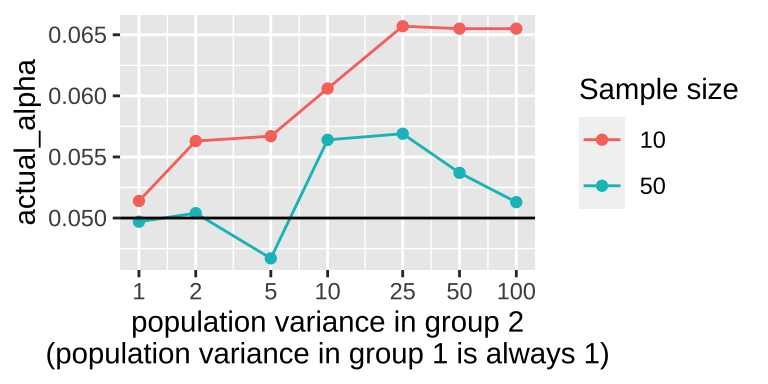
The plot shows that violating the assumption of equal variance seems to matter most when sample size is small and violations are extreme.
25.7 Quiz
25.8 Boring math
You don’t need to know this, but the formula for Welch’s t-test is
\[t\quad =\quad {\;\overline {X}_{1}-\overline {X}_{2}\; \over {\sqrt {\;{s_{1}^{2} \over N_{1}}\;+\;{s_{2}^{2} \over N_{2}}\quad }}}\,\]
With degrees of freedom equal to
\[{\displaystyle df \quad \approx \quad {{\left(\;{s_{1}^{2} \over N_{1}}\;+\;{s_{2}^{2} \over N_{2}}\;\right)^{2}} \over {\quad {s_{1}^{4} \over N_{1}^{2}\times df _{1}}\;+\;{s_{2}^{4} \over N_{2}^{2} \times df _{2}}\quad }}}\]