Chapter 4 Handling data in R

This is a lot getting started, remember our goal here is exposure, not mastery. Mastery will come as the term progresses.

Motivating scenarios: We just got our data, how do we get it into R and explore?

Learning goals: By the end of this chapter you should be able to get data into R and explore it. Specifically, students will be able to:

• Load data into R and make their own tibbles.
  
• filter, mutate, arrange, and select data with the dplyr package.
  
• (Optional) Tidy data with the tidyr package.

There is no external reading for this chapter, but

• Watch the required videos from Stat 545 – one about using dplyr and about tidying data embeded in the text (feel free to skip the videos featuring me), and
• Complete the learnR tutorials and quizes embeded in this chapter.
  
• And canvas assignment which goes over the quiz, readings, tutorials and videos.

4.1 Intro

Through the rest of this chapter we will buy in fully to the tidyverse, so make sure it’s installed and load it at the top of your script by typing and entering library(tidyverse). In the next portions of this section, we focus on how to load and process data with tidyverse tools in R.

But first, we describe the primary structure that holds data in the tidyverse, a tibble. A tibble is a data structure in which each column is a vector and (ideally) entries in a row are united by relating to the same observation (e.g. individual at a time). Each variable associated with an observation is a column (i.e. a vector), and all so while all entries in a column must be of the same class, each column in a tibble can have its own class. Tibbles do not ensure that our data are tidy but they do make this easier.

If you have spent time in base R you are likely familiar with matrices, arrays, and data frames - don’t even worry about these. A tibble is much like a data frame, but has numerous features that make them easier to deal with. If you care, see chapter 10 of R for Data Science (Grolemund and Wickham 2018) for more info. Anyways, in this course we will focus on vectors and tibbles, ignoring arrays and matrices, and avoiding lists for as long as possible.

4.1.1 First primer

Now is a great time to complete the Primer on tibbles, embedded below (Fig. 4.1).

Figure 4.1: The RStudio Primer on tibbles

4.2 Getting Data into R

Getting data into R is often the first challenge we run into in our first R analysis. The video (Fig: 4.2) and text below should help you get started.

Figure 4.2: Getting data into R (6 in and 6 seconds).

4.2.1 Loading data

Ideally, your data are stored as a .csv, and if so you can read data in with the read_csv() function. R can deal with other formats as well. Notably, using the function readxl::read_excel() allows us to read data from Excel, and can take the Sheet of interest as an argument in this function.

Here’s an example of how to read data into R.

library(tidyverse)
toad_data <- read_csv(file = "science_projects/Toads/data/toad_data.csv")

The bit that says science_projects/Toads/data/ points R to the correct folder, while toad_data.csv refers to the file we’re reading into R and assigning to toad_data. Using tab-completion in RStudio makes finding our way to the file less terrible. But you can also point and click your way to data (see below). If you do, be sure to copy and paste the code you see in the code preview into the script so you can recreate your analysis..

As above, best practices for loading data make use of R projects, so feel free to learn more. But for now, we’re focused on good enough practices.

4.2.2 Entering data into R

We can create tibbles manually. I present the simplest and most common way this is done.

toad_data <- tibble(             # This makes the data
  individual = c("a", "b", "c"),
  species    = factor(c("Bufo spinosus", "Bufo bufo", "Bufo bufo")),
  sound      = c("chirp", "croak","ribbit"),
  weight     = c(2, 2.6, 3),
  height     = c(2,3,2)
) 

toad_data                        # This shows the data

## # A tibble: 3 x 5
##   individual species       sound  weight height
##   <chr>      <fct>         <chr>   <dbl>  <dbl>
## 1 a          Bufo spinosus chirp     2        2
## 2 b          Bufo bufo     croak     2.6      3
## 3 c          Bufo bufo     ribbit    3        2

Feel free to read about more ways to make tibbles if you desire. Many of these options are fun and useful, but a distraction from our major mission

4.3 Dealing with data in R

Figure 4.3: Watch this video introducing dplyr (watch the frist 5 min and 9 sec), from STAT 545 – a grad level data science class at the University of British Columbia. We will borrow from this course occasionally.

Looking at the toad.data tibble above, we can get a sense of the utility of a tibble. We can see, not only the first few values of the data set, but also the class of each variable (chr for character, fct for factor, dbl for double – a continuous class of data).

4.3.1 Viewing and glimpsing tibbles

To see the entire dataset in a spreadsheet, type view(toad_data). While this is not useful for the small toad_data we made, it could be more useful for the starwars data set already in tidyverse. Have a look with view(starwars).

The glimpse() function is another useful way to explore a new, large data set. For example

While these are among the very handy tidyverse functions, the real utility of tidyverse is that it gives us a unified way to deal with data. Usually when we get data we want to handle/clean it, summarize it, visualize the results and develop a statistical model from it. This is where tidyverse really shines!

We first focus on handling data with the dplyr package. Today we’ll talk about using it to filter, arrange, and mutate our data, and to select columns of interest.

Figure 4.4: From R for data Science (Grolemund and Wickham 2018)

I say this all the time but: learning dplyr + ggplot was one of the highest payoff things I've done in my career.

— Joshua G. Schraiber🌹 (@jgschraiber) January 22, 2019

4.3.2 mutate your data

In our toad_data, we have height and weight. Let’s add a column for BMI (weight divided by height) with the mutate() function.

toad_data <- mutate(toad_data, BMI = height / weight)
toad_data

## # A tibble: 3 x 6
##   individual species       sound  weight height   BMI
##   <chr>      <fct>         <chr>   <dbl>  <dbl> <dbl>
## 1 a          Bufo spinosus chirp     2        2 1    
## 2 b          Bufo bufo     croak     2.6      3 1.15 
## 3 c          Bufo bufo     ribbit    3        2 0.667

4.3.3 arrange rows

You might want to sort BMI from lowest to highest, or vice-versa. The arrange() function is here for you!

arrange(toad_data, BMI)       # arrange from lowest to highest

## # A tibble: 3 x 6
##   individual species       sound  weight height   BMI
##   <chr>      <fct>         <chr>   <dbl>  <dbl> <dbl>
## 1 c          Bufo bufo     ribbit    3        2 0.667
## 2 a          Bufo spinosus chirp     2        2 1    
## 3 b          Bufo bufo     croak     2.6      3 1.15

arrange(toad_data, desc(BMI)) # arrange from highest to lowest

## # A tibble: 3 x 6
##   individual species       sound  weight height   BMI
##   <chr>      <fct>         <chr>   <dbl>  <dbl> <dbl>
## 1 b          Bufo bufo     croak     2.6      3 1.15 
## 2 a          Bufo spinosus chirp     2        2 1    
## 3 c          Bufo bufo     ribbit    3        2 0.667

4.3.4 filter your data

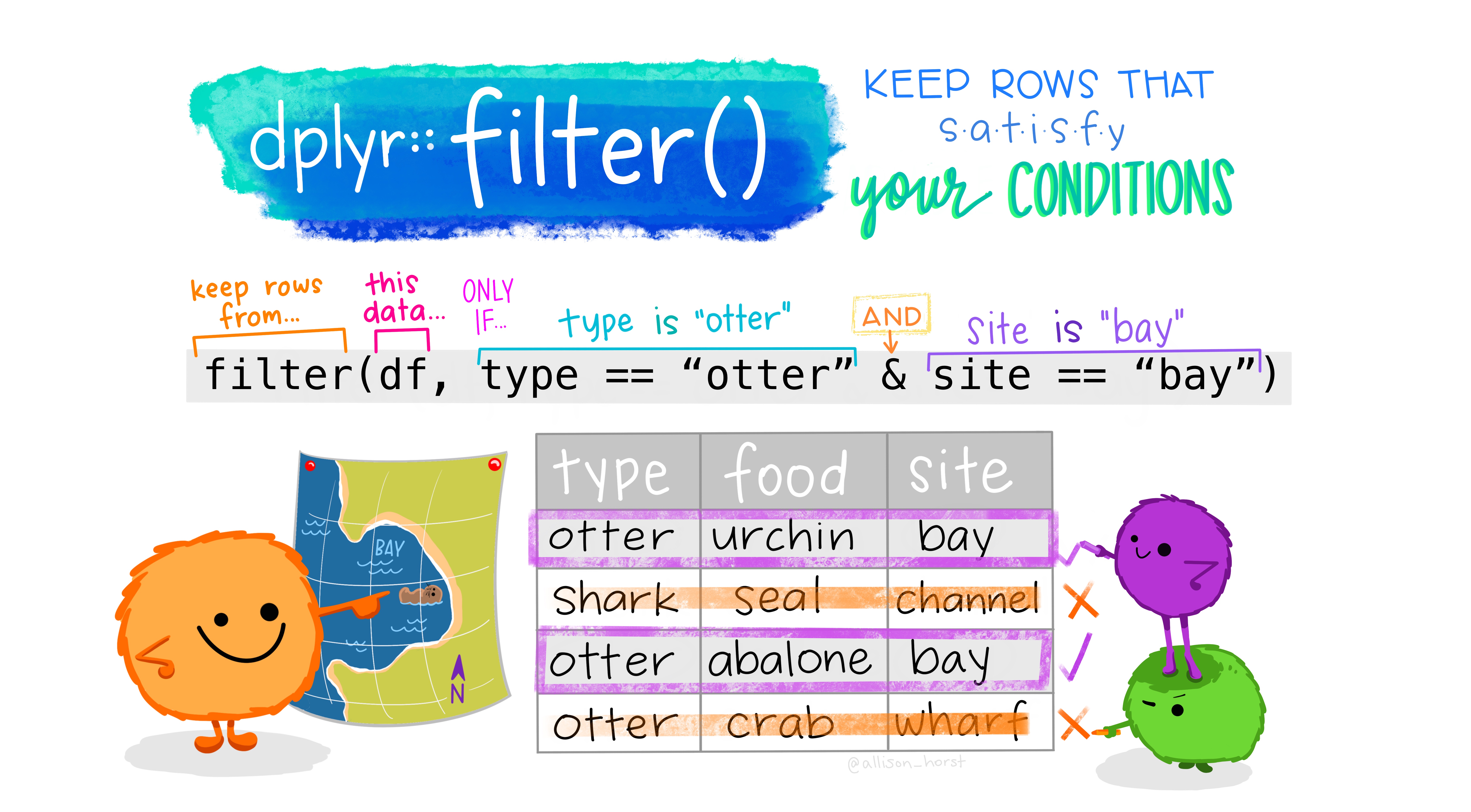
Say we only wanted to deal with individuals of the species, Bufo bufo. We can filter() our data to only have them!

filter(toad_data, species == "Bufo bufo" )

## # A tibble: 2 x 6
##   individual species   sound  weight height   BMI
##   <chr>      <fct>     <chr>   <dbl>  <dbl> <dbl>
## 1 b          Bufo bufo croak     2.6      3 1.15 
## 2 c          Bufo bufo ribbit    3        2 0.667

We can filter by any set of logical questions like greater than >, greater than or equal to >=, less than <, not equal !=, in a vector %in% etc… (see Ch 3 for more info).

4.3.5 select your columns

Let’s say we didn’t care about the height or weight, and we just wanted individual, species, sound, and BMI. We can select() those columns as follows:

dplyr::select(toad_data, individual, species, sound, BMI)

## # A tibble: 3 x 4
##   individual species       sound    BMI
##   <chr>      <fct>         <chr>  <dbl>
## 1 a          Bufo spinosus chirp  1    
## 2 b          Bufo bufo     croak  1.15 
## 3 c          Bufo bufo     ribbit 0.667

A negative sign in select means remove, so select(toad_data, -height, - weight) will give the same result as the code above.

dplyr::select(toad_data, -height, -weight)

## # A tibble: 3 x 4
##   individual species       sound    BMI
##   <chr>      <fct>         <chr>  <dbl>
## 1 a          Bufo spinosus chirp  1    
## 2 b          Bufo bufo     croak  1.15 
## 3 c          Bufo bufo     ribbit 0.667

4.3.5.1 pull() vectors from tibbles

Some things we do in R require vectors to be pulled out of tibbles. We can achieve this with the pull() function. For example, to get the BMI as a vector, type

pull(toad_data, var = BMI)

4.3.6 Second primer

Now is a great time to complete the Primer on isolating data with dplyr, embedded below (Fig. 4.5).

Note - we won’t be working on the last part %>% aka ‘piping’ until next class so, you can out that off for a few days.

Figure 4.5: The RStudio Primer on isolating data with dplyr

4.4 Tidying messy data

Figure 4.6: Tidy tools require tidy data

In Ch. 2, we saw that it is best to keep data in a tidy format, and in Section 3.2.2 we noted that Tidyverse tools have a unified grammar and data structure. From the name, tidyverse, you could probably guess that tidyverse tools require tidy data – data in which every variable is a column and each observation is a row. What if the data you loaded are untidy? The pivot_longer function in the tidyr package (which loads automatically with tidyverse) can help! Take this example dataset, about grades in last year’s course.

## # A tibble: 2 x 4
##   last_name first_name exam_1 exam_2
##   <chr>     <chr>       <dbl>  <dbl>
## 1 Horseman  BoJack       35     36.5
## 2 Carolyn   Princess     48.5   47.5

This is not tidy. If it were tidy each observation would be a score on an exam. So we need to move exam to another column. We can do this!!!

tidy_grades <-pivot_longer(data = grades, # Our data set
             cols = c(exam_1, exam_2),    # The data we want to combine
             names_to = "exam",           # The name of the new column in which we put old names.
             values_to = "score"          # The name of the new column in which we put the values.  
             )

tidy_grades

## # A tibble: 4 x 4
##   last_name first_name exam   score
##   <chr>     <chr>      <chr>  <dbl>
## 1 Horseman  BoJack     exam_1  35  
## 2 Horseman  BoJack     exam_2  36.5
## 3 Carolyn   Princess   exam_1  48.5
## 4 Carolyn   Princess   exam_2  47.5

This function name, pivot_longer, makes sense because another name for tidy data is long format. You can use the pivot_wider function to get data into a wide format.

Learn more about tidying messy data in Fig. 4.7:

Figure 4.7: Tidying data (first 5 min and 40 seconds are relevant).

4.5 Think about reproducibility

Science is iterative, social / collaborative, and builds on previous work. You should know that

1. Your first analysis is almost never your last.
   
2. Your will need to be able to explain EXACTLY what you did to others.
   
3. People might want to take you’ve done, understand it, and do it again on this or another data set, perhaps changing it a bit.

Think about this when you work in R. I suggest asking yourself the following questions:
(1) Could I explain what my code is doing to a colleague? What if I hadn’t looked at it in a month? Could someone who’s pretty good with R look at my code and understand what I was trying to do?
(2) Could my code work well (within minimal changes) on another data set? How about on another computer?
If your work is fully reproducible, the answers should all be yes.

One of the great things about scripting-based analyses that you can do in R (or similar programs) is that it facilitates us answering “yes” to most of these questions — take advantage of this. Always save your R script. Use enough commenting (#) to make sure it makes sense. Make sure it works from start to finish without anything in your R environment. etc…

Assignment

1. Complete RStudio’s primers on working with tibbles and isolating data with dplyr

2. Complete the glimpse intro (4.3.1) and the quiz (4.5.1).

3. Fill out the quiz on canvas, which is very simlar to the one below.

4.5.1 Quiz

You know the drill… on canvas

4.6 Functions covered in Collecting and storing data + handling and visualizing it in R

All require the tidyverse package

4.6.1 Functions for loading, formatting, and exploring data

tibble(): Entering data as a tibble. Give each column a name and assign its values with an equals sign, =. Separate columns with a comma ,.
glimpse(): Show the name of every column in your data frame, as well as their class and first few values.
view(): Look at your entire tibble as a scrollable spreadsheet.
read_csv(): Reads a dataset saved as a .csv into R.
readxl::read_excel(): Reads a dataset saved as a .xlsx into R. You can also specify the sheet with sheet =.
pivot_longer(): Allows use to tidy data.
pivot_wider(): Allows use to go from tidy to wide data.

4.6.2 Functions for dealing with data

mutate(): Add a new column, usually as some function of existing columns.
arrange(): Sort rows from low to high (or from high to low with arrange(desc())) values of a specified column.
filter(): Limit your dataset to those with certain values in specifed columns.
select(): Select columns of interest (or remove ones you do not care about with select(-)) from your tibble. ```

4.6.3 dplyr cheat sheet

There is no need to memorize anything, check out this handy cheat sheet!

Figure 4.8: download the dplyr cheat sheet

References

Grolemund, Garrett, and Hadley Wickham. 2018. “R for Data Science.” https://r4ds.had.co.nz/.