Chapter 3 Day one of R and RStudio
Motivating scenario: Motivating scenario: You have heard about R and RStudio, and maybe used them, but want a foundation so you can know whats going on as you do more and more with it.
Learning goals: By the end of this chapter you should be able to
- Explain why we are using R and RStudio.
- Describe the five tips for writing code like a pro.
- Install R and RStudio (or have access to them on RStudio cloud).
- Set up RStudio preferences.
- Install the tidyverse package.
- Open and save an R script.
- Explain vectors, classes of variables, doing math, and asking logical questions in R.
3.1 What is R and why / how do we use it?
R is a computer program, which is the go to language for most statisticians and data scientists (although some prefer python or Julia). R makes it possible to conduct complex statistical analyses, make nice figures, and write this book, all in one environment.
As opposed to GUI’s, like Excel, or click-based stats programs, R is focused around writing and sharing scripts. This allows analyses to be shared and replicated, ensures that data manipulation occurs in a script, preserving the integrity of the original data, and allows for tremendous flexibility.
3.2 Why use R?
- R is free.
- There are many “packages” in R for specialized analyses.
- R can make nice graphics.
- While learning R is not easy, inexperienced programmers can quite quickly do useful things. You will be able to make nice plots and summarize data by next week!
- Using R (or any scripting based analysis) allows us to save all the steps of our analysis, making our work easy to reproduce, describe, and build off of.
Figure 3.1: Watch this video about why and how to R (6 min and 10 sec), from STAT 545 – a grad level data science class at the University of British Columbia. We will borrow from this course occasionally.
3.2.1 What is RStudio?
More precisely, R is a programming language that runs computations, while RStudio is an integrated development environment (IDE) that provides an interface by adding many convenient features and tools. So just as the way of having access to a speedometer, rearview mirrors, and a navigation system makes driving much easier, using RStudio’s interface makes using R much easier as well.
In addition to being a great place to use R, RStudio is a Certified B corporation, which offers many great resources we will rely on over this term. RStudio has a freemium business model, and you will not need to pay for any of RStudio’s products this term.
3.2.2 What is the tidyverse?
A great part about R is that many people have written packages to help with specific tasks.
The tidyverse refers to both a set of packages, and a way to do things in R. The tidyverse packages we use the most in this course are:
ggplot2: For making plots.
dplyr: For summarizing and handling data.
tidyr: For converting data from wide to long format (and vice versa).
readr: For reading in data.
forcats: For controlling the order of categorical variables.
We will use the tibble, stringr, and purrr packages less often if at all (although I use them often). If you are using your computer, rather than RStudio Cloud, you will need to install tidyverse (see 3.2.3) the first time you use it.
![The tidyverse is an opinionated collection of R packages... shar[ing] an underlying design philosophy, grammar, and data structures. - [tidyverse.org](https://www.tidyverse.org/)](images/tidyverse.jpeg)
Figure 3.2: The tidyverse is an opinionated collection of R packages… shar[ing] an underlying design philosophy, grammar, and data structures. - tidyverse.org
You will see that there are many ways to do things in R. Over years of teaching this course I have switched to teaching predominantly using tidyverse tools.
One major reason for this is that the focus on a shared and coherent philosophy, grammar and data structure makes the tidyverse easier to teach and learn than base R. However, there are still challenges to learning and teaching the tidyverse, the two major challenges are
- It takes time to learn and appreciate the shared philosophy and data structure.
- Many people first learned R using base R, so it can be frustrating to start to learn again.
Overcoming challenge (1) takes time but is helped by reflecting on why and how code works when it works, and fails when it fails (rather than copying and pasting code that works), and continually asking questions.
Overcoming challenge (2) can be tough, but I believe it’s well worth it. Amelia McNamara’s R syntax comparison cheat sheet (Fig: 3.3) can help .
](https://d33wubrfki0l68.cloudfront.net/948e2a62a1eab719f3cad4763d74b383ed466acc/d4baa/wp-content/uploads/2018/02/syntax.png)
Figure 3.3: download the syntax comparison cheat sheet
3.3 3.2 Installing R and tidyverse (or not)
We use R version 4.0.0 or above, and tidyverse version 1.3.0 or above.
You can either download and install R, RStudio, and tidyverse onto your computer (see Installing RStudio for more info), or you can do all the coursework with RStudio Cloud without installing anything on your computer (see Getting on RStudio Cloud for more info). Which option is right for you? It depends (see below). I suggest doing both and seeing which you prefer.
3.3.1 Getting on RStudio Cloud
Using RStudio Cloud allows you to use R and RStudio without installing anything on your computer. Additionally, if you log into our course project on RStudio Cloud you will not need to install any packages or load any files except those you want for fun or for your independent project at the end of term.
Advantages to RStudio Cloud
From my experiencing teaching this course, about 5% of students have computers or computer systems where installing R is challenging, now you don’t have to.
Some students have older computers with limited computation. For them, a few class exercises (involving large-scale permutation or simulation) go super slow, and they can get justifiably frustrated.
Some computer setups make installing tidyverse or other specific R packages somewhat painful. RStudio Cloud removes this pain.
Using the course project guarantees that you’ll get the same environment as the prof and TA, making it easier for them to help you.
Disadvantages to RStudio Cloud
- The biggest disadvantage of RStudio cloud is that it’s expensive if we all use it and I only paid for a certain amount of usage, so please use it only if you’re having issues using R on your computer. Please e-mail me f you would like to use it!
- Sometimes the system can get overwhelmed. This is pretty rare, but once a student was trying to use RStudioCloud during the international RStudio convention. The RStudio Cloud could not handle all the traffic and went down that day.
- You need an internet connection to use R. This can be a bummer if you don’t always have a reliable one.
- Some people (🖐) like having everything on their computer and struggle thinking about / working with folders on a cloud.
- Using the course project on RStudio Cloud might prevent you from learning how to load data, download packages etc.
3.3.2 Installing RStudio
First download/update R from here, be sure to download the version compatible with your computer, and pick any CRAN mirror you like (I usually do Iowa). If you installed R a while ago, be sure you’re using R version 4.0.0 or above.
Then download/update RStudio from here. Be sure to select he free version (RStudio Desktop, Open Source License), and as above, be sure to download the version compatible with your computer. If you installed RStudio a while ago, be sure you’re using RStudio version 1.3.0 or above.
I installed RStudio.
— Joanne August (@joanneXaugust) September 17, 2020
I am Data Scientist now. #AcademicTwitter #phdchat #phdlife pic.twitter.com/UaYspg9MRF
Advantages to downloading and installing RStudio
- You can do a bunch without stable internet.
- You are not reliant on a cloud service which could go down.
- Everything is on your computer.
- You learn the joys (and frustrations, and how to overcome them) of dealing with packages, loading data etc… .
Disadvantages to downloading and installing RStudio
3.3.3 Installing tidyverse
Open RStudio and type install.packages("tidyverse") into the console, and then library(tidyverse) to ensure this worked.
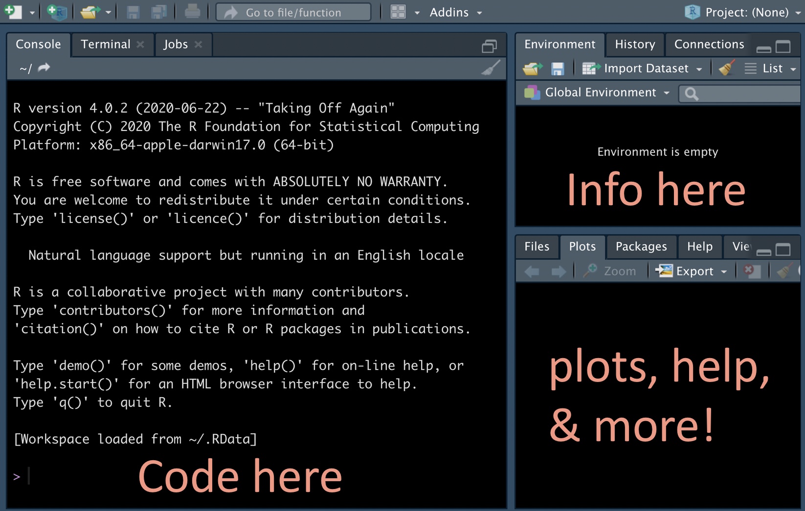
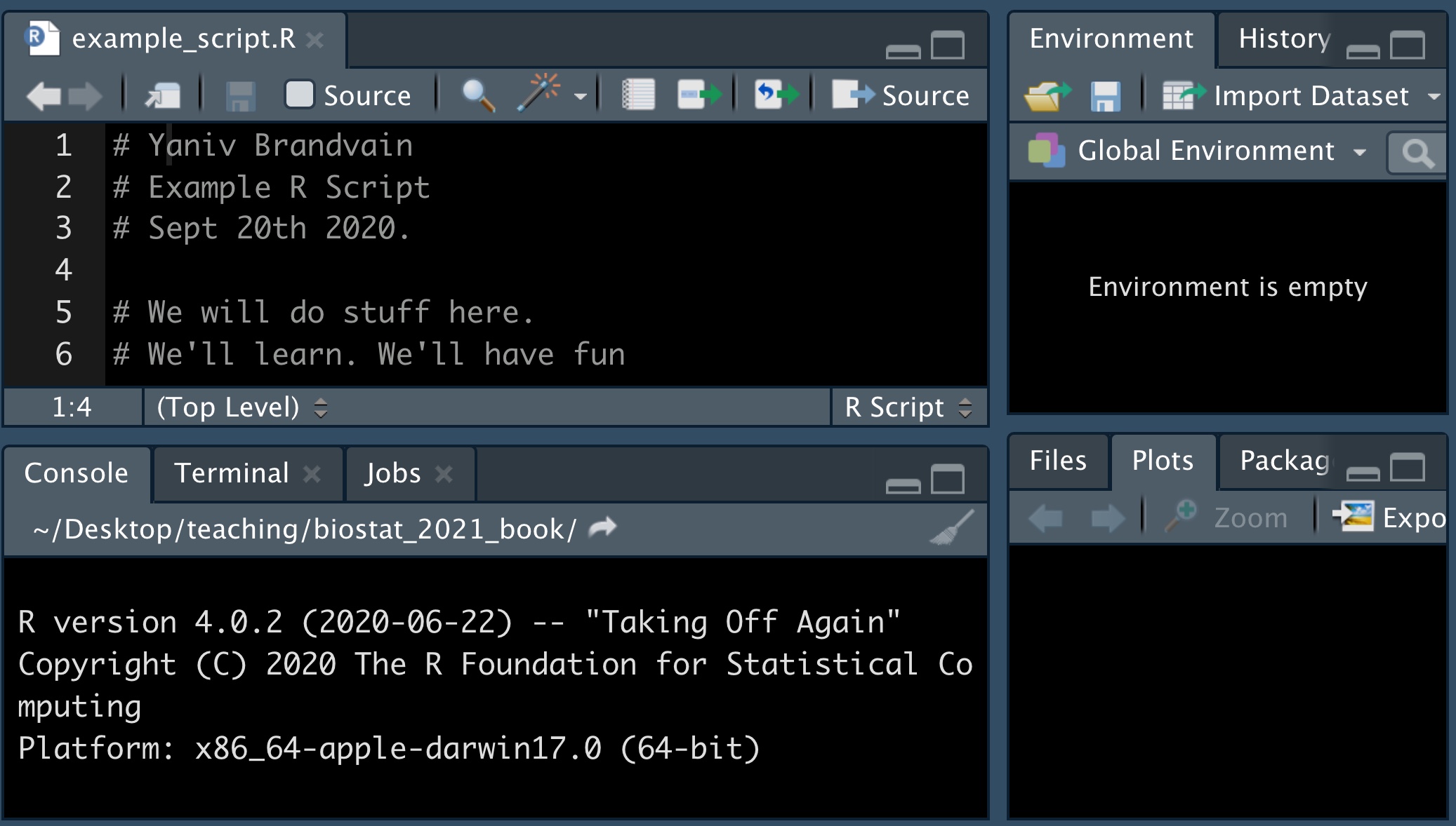
3.4 The RStudio IDE
3.4.1 A tour of the RStudio IDE.
If you are unfamiliar with the RStudio environment you should watch this video on the RStudio webpage.
Figure 3.4: The RStudio IDE Overview (2min and 45 sec)
3.4.2 A tour of the Rstudio environmenmt
Customize settings and preferences in the RStudio IDE.
Suggested preferences for RStudio IDE.
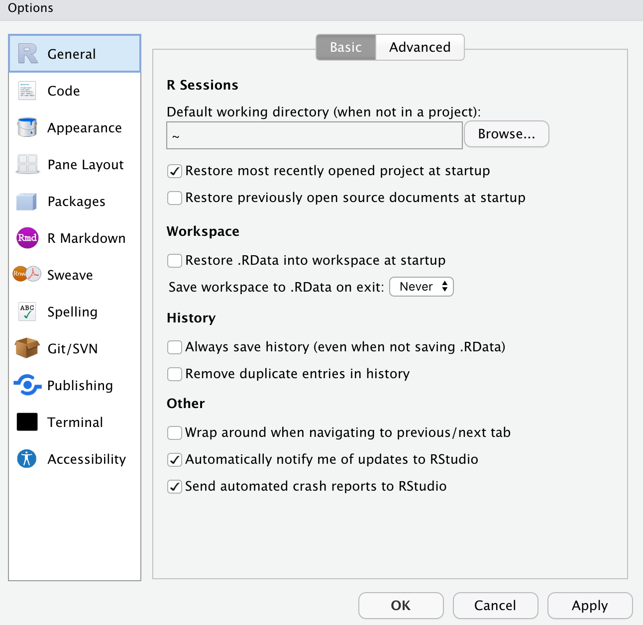
Figure 3.5: Suggested preferences for RStudio IDE.
After you open RStudio, navigate to Preferences under the RStudio tab. Set yours to be like mine (Fig: 3.5), below and then click apply.
Feel free to set Code, Appearance, Pane Layout etc to however you like!
3.5 Intro to R
3.5.1 Using R as a calculator and for logical questions
We can use R for doing math. For example:
1 + 1will return 2,
3 * 2will return 6,
3 / 2will return 1.5,
3^2will return 9, etc… .
We can also use R for asking logical questions. For example:
- ‘Is one greater than two?’ like this
1 > 2, which returnsFALSE.
- ‘Does four divided by four equal one?’ like this
4/4 == 1(note the two equals signs), which returnsTRUE.
- ‘Does four divided by four not equal one?’ like this
4/4 != 1(note an exclamation point, then an equals sign), which returnsFALSE.
- ‘Is four divided by four less than or equal to one?’ like this
4/4 <= 1(note an less than sign followed by the equals sign), which returnsTRUE.
- ‘Is four divided by four greater than or equal to one?’ like this
4/4 >= 1(note an greater then sign, then an equals sign), which returnsTRUE.
3.5.2 Vectors in R
Most of what we do in R starts with a vectors – a combination of simple entities. We already came across a few simple vectors of length one – for example, the number, 1 and the logical statement, TRUE, above.
Vectors are often longer than length one, for example, we can make a vector with the numbers one, five, and two with the c()oncatenate function as follows c(1, 5, 2) which returns 1, 5, 2.
Classes of Vectors in R
All entries in a vector must be of the same class. The three most relevant classes are:
numeric– Contains numbers which can take any value. For examplec(1, 2, 3)returns1, 2, 3.
logical– Contains logical statements. For example,c(TRUE, FALSE, FALSE)returnsTRUE, FALSE, FALSE.
character– Contains letters, words, and/or phrases. For examplec("The dog", "jumped", "over", "the moon")returnsThe dog, jumped, over, the moon.
You may also come across two other classes of vectors:
factor– This is a lot like a character, with the caveat that they are coded by numbers in R’s brain (see below). This can sometimes make things tough, so be careful, and consider when things are not working right that maybe you have factor when you thought you had a character.
integer– A number that must take an integer value. For exampleas.integer(c(1, 2.1, 3))returns1, 2, 3.
Using math and/or logical operations on vectors
In R you can add, subtract etc. two vectors. When doing so make sure vectors are of the same length, or one is of length one, otherwise you can get weird results.
- To add one to the vector
1, 2, 3, type1 + c(1, 2, 3)to get2, 3, 4.
- Similarly, to multiply the vector
1, 2, 3, by two, type2 * c(1, 2, 3)to get2, 4, 6.
- To divide the vector
1, 2, 3by the vector2, 4, 1, typec(1, 2, 3) / c(2,4,1), which returns0.5, 0.5, 3.
- To ask, for each element in the vector
1, 2, 3, if it equals one, typec(1, 2, 3) == 1, which returnsTRUE, FALSE, FALSE.
- To ask, for each element in the vector
1, 2, 3, if it equals the corresponding element in the vector3, 2, 1, typec(1, 2, 3) == c(3, 2, 1), which returnsFALSE, TRUE, FALSE.
3.5.3 Using functions in R
Only so much can be done with simple math. We can do more complex analyses in R with functions. Functions take in arguments and return some output. Here are some simple examples:
- To get the mean of a vector, use the
mean()function. For example, mean(x = c(1, 2, 3))returns2.
- To get the length of a vector, use the
length()function. For example,length(x = c(1, 2, 3))returns3.
- Use the
help()function to learn more about a given function. For examplehelp(length)will return this (Fig: 3.6).
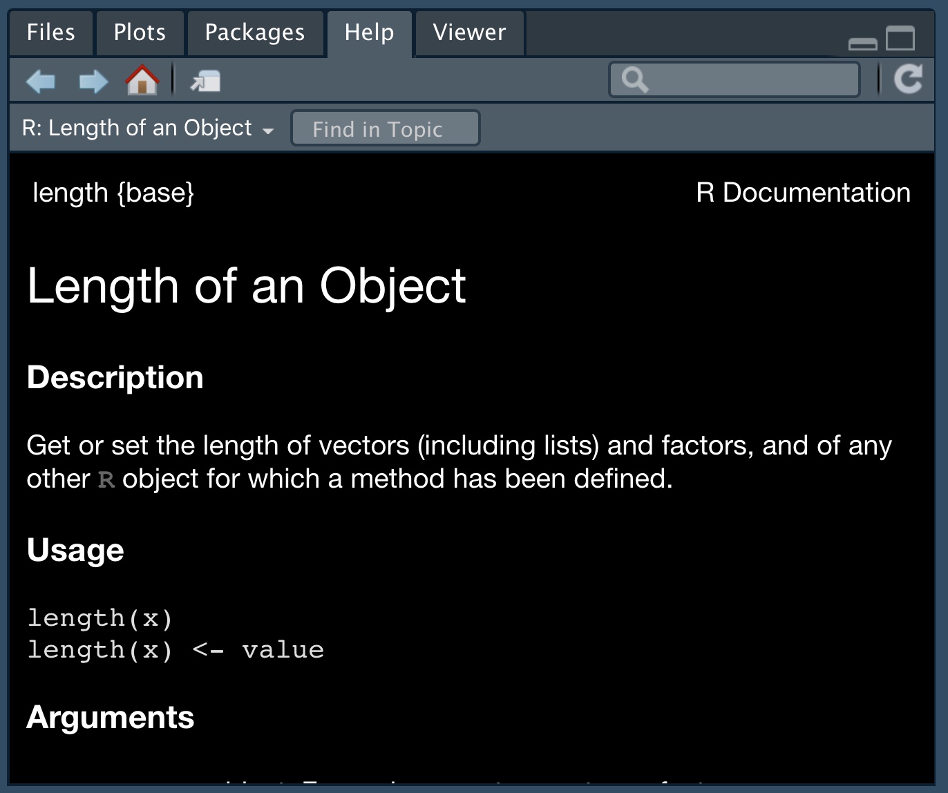
Figure 3.6: An example of R help
Throughout the text, I include a hyperlink to the help for every function I introduce. There is no need to look into all of these, but it is a good practice to look at the when you are confused. Unfortunately it takes a bit of practice / knowledge to make sense of R’s help. So, check out this reference to figure out how to get the most from R’s help.
The tab button is very useful when we deal with functions. Hitting tab as you begin to type a function’s name will give suggested functions, with a brief description, while hitting tab inside the parentheses of a function will show the arguments the function takes.
sqrt(x = 4), returns 2, as does sqrt(4). But it’s usually a good practice to do so, especially when there are more than two arguments as this makes it easier to understand your code and harder to mess up.
3.5.4 Assigning variables in R
Use the assignment operator <- to assign values to a variable. For example
num_vec <- c(4, 9, 16)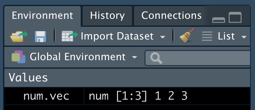
With these variables assigned, we can do simple math, ask logical questions , use them as arguments for functions. For example sqrt(x = num_vec) returns 2, 3, 4. Note, this is the same as typing sqrt(num_vec) and with just one argument (x) for the function, this is totally unnecessary. When there are more arguments it is good practice to include the argument name and the equals sign, as this makes code easier to read, and more likely to work (otherwise R assumes we put things in a specific order).
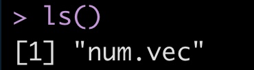
All variables assigned should be in your environment window, or you can use the ls() function to ask R for them.
Converting between types of vectors
logicaltonumeric– A convenient trick in R is thatTRUEequals one andFALSEequals zero. Sosum(c(TRUE, FALSE))returns1, andmean(c(TRUE, FALSE))returns0.5.
factortocharacter(and vice versa) – This usually works without incident, so you can convert a factor,factor_vec <- factor(c("a","x")), to a character like this:char_vec <- as.character(factor_vec).
factortonumeric– This will return the numeric ID associated with levels, soas.numeric(factor_vec)returns1, 2.
numerictofactor– DON’T DO THIS, UNEXPECTEDLY BAD THINGS WILL HAPPEN.
3.5.5 Writing R scripts and beyond
A great thing about R is that you can remember and share exactly what you have done by saving your work as a script. In doing so it’s best practice to type your name, date and the goal of the analysis at the top (with a # to tell R this isn’t code), plus a description of your goals. Regular comments throughout, help make your code more usable.
To make a new R Script, click on File, then New File, and then R Script.
3.6 Loading tidyverse and other packages
In Section 3.2.2 we introduced the idea that people have developed packages to extend R to do a bunch of stuff, and in Section 3.2.3, we saw that we install an R package with the install.packages() function.
We only need to install a package once, but we need to load all packages we are using every time we open a new R session. Use the library() function to do so.
So, for example, type the following to load the tidyverse package
You should see messages like I did upon loading the tidyverse library. You should also see in the Packages tab, that you now have a check next to dplyr, forcats, ggplot2, purrr, readr tibble, and tidyr, as these are all loaded with tidyverse.
3.7 Preparing for success
Follow these Rules to help make this class and your life easier.
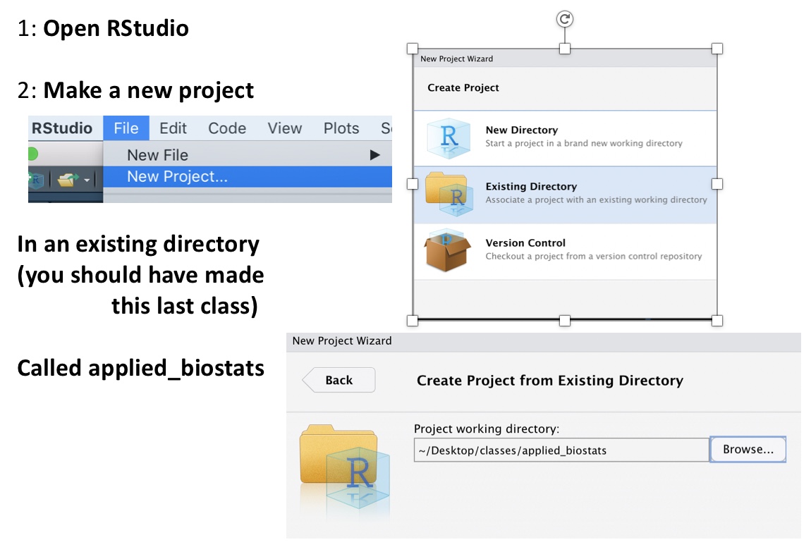
Today!
- Make a folder for this course and include a subfolder called data (as I said in the last chapter).
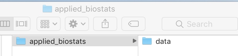
- Open
Rright now and make a project calledapplied_biostatsin the existing folder,applied_bioststats.
Everyday for class homework etc!
Double click the
applied_biostats.Rprojto open RStudio, rather than opening RStudio directly (or if you insist, open the project after you open RStudio).Open a new script.
Write the date and what we are working on in a comment (that is, after a hash
#)Load all packages you will need (almost always tidyverse, sometimes more)
Before doing anything else, save the script in your applied_biostats folder with a nice name (e.g.
class_02_intro_to_R.R).Go do your thing!
#  Jane 21 2021
#  Good practces
library(tidyverse)
3.8 Observations and suggeastions for learning R / computer stuff
Teaching this class for years, I’ve learned a few things about leaning R that you should know.
3.8.1 Observations
- Some people pick R up fast, other slowly.
- The speed at which students get familiar with R is unrelated to intelligence.
- Everyone who keeps trying gets there eventually.
- Despair and feeling low/dumb are the things that get people jammed up.
3.8.2 Suggestions
- Don’t worry. Keep trying. But TAKE BREAKS.
- Step away from the computer as much as possible, code & make plans on scratch paper.
- Be patient & understanding with yourself and your friends.
- Be creative.
- Ask for help.
- When something works (or it doesn’t) take time to figure out how / why.
- Fight the urge to compare yourself (negatively or positively) to others.
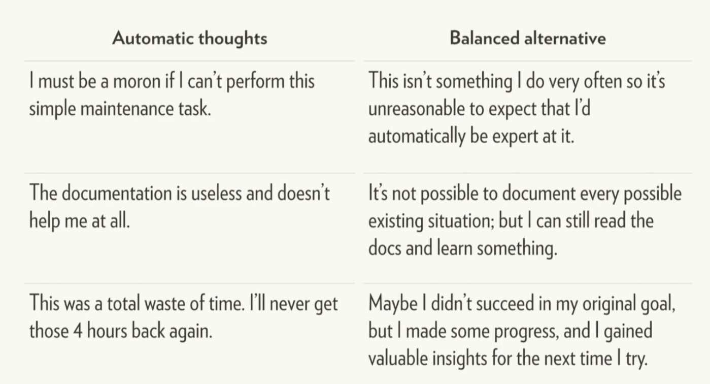
Today at the RStudio conference, Hadley Whickham, conrasted the “automatic negative thoughts” we feel some time in coding to the “balanced alternative” that we want to get to.
3.9 RStudio primer
Be sure to complete this primer from RStudio. This will get you a solid foundation in R which we will build off in the coming weeks.
Figure 3.7: Primer on programming basics: Complete the RStudio programming basics tutorial from the RStudio website
3.10 Intro to R and RStudio: Quiz
Complete the quiz below, a nearly identical quiz will be on canvas.