13 Transforming data

Anyone regularly working with data is aware that transforming data (aka. “data munging” or “data wrangling”) is an essential pre-requisite for any successful data analysis.

The task of transforming data can be further decomposed into reducing or reshaping data. Our main focus in the current chapter lies on reducing data (by creating chains of functions that allow answering questions about the contents of a dataset). By contrast, the next Chapter 14 will primarily focus on reshaping data (by turning “messy” into “tidy” tables).

Key topics (and corresponding R packages) of this chapter are:

• Section 13.2: The pipe operator from magrittr (Bache & Wickham, 2022)

• Section 13.3: Transforming tables with dplyr (Wickham, François, et al., 2023)

Both these sections and packages are designed for manipulating data structures (mostly vectors or tables) into other data structures (more vectors or tables). Although transforming data can be viewed as a challenge and a task in itself, our primary goal usually consists in gaining insights into the contents of our data.

Preparation

Recommended readings for this chapter include

• Chapter 3: Transforming data of the ds4psy book (Neth, 2023a)

• Chapter 5: Data transformation of the r4ds book (Wickham & Grolemund, 2017)

Preflections

Before reading, please take some time to reflect upon the following questions:

• Assuming we had all the data required for answering our question, which additional obstacles would we face?

• In which data structures are the answers to our data-related questions represented?

• Do answers to our data-related questions always contain the entire data? Or do we typically select and reduce data, so that it becomes impossible to reconstruct the data from our answers?

13.1 Introduction

Data transformations and the corresponding functions can be classified into two general types:

1. Reducing operations are data transformations that typically modify both the shape and content of data. Examples of data reductions include sampling values from a population, describing a set of values by some measure (e.g., its mean or median), or computing some summary measure out of a set of values (e.g., to learn about a test’s sensitivity or positive predictive value).

2. Reshaping operations modify the shape or structure of data without changing its contents. When re-shaping data, some shapes are more suitable for further analysis than others. A particular form of tabular data can be described as tidy data. Typical examples for reshaping data include transforming the values of a vector into an array or matrix, or re-arranging the rows or columns of a table.

Thus, whereas reshaping operations can be reversed, reducing data usually goes beyond mere “trans-formation” by being uni-directional: We typically cannot reconstruct the original data from reduced data.

13.1.1 Practice: Reshape or reduce?

Assuming the following vectors v and a:

v <- 1:9
a <- sample(c("A", "B", "C"), 10, replace = TRUE)

do the following operations reduce or reshape these data structures? Why?

Hint: Evaluate the expressions in order to see their results.

matrix(v, nrow = 3)
mean(v)
data.frame(nr = v, freq = v) %>% 
  group_by(nr) %>%
  count()

rev(a)
table(a)
a == "A"

13.1.2 Key concepts

In addition to introducing three popular tidyverse packages, this chapter introduces some terminology for talking about data transformations:

• In discussing different data transformations, we distinguish between reshaping and reducing data;

• Key concepts of Sections 13.2 and  include the pipe operator (from the magrittr package);

• Section 13.3 introduces concepts to filter, select, and mutate variables, and group and summarize data (from the dplyr package).

What data structures are being transformed? While both types of data transformations can be demonstrated with vectors, we typically operate on entire data tables. Working with a table (as inputs to functions) typically yields new tables (as outputs of functions). This is where the pipe operator %>% from the magrittr package (Bache & Wickham, 2022) comes into play: It passes (or “pipes”) the result of one operation (i.e., the output of a function) as an input to another operation (i.e., as the first argument of another function).

13.2 The pipe from magrittr

The dplyr R package is awesome.
Pipes from the magrittr R package are awesome.
Put the two together and you have one of the most exciting things to happen to R in a long time.

Sean C. Anderson (2014)

The pipe operator from the magrittr package (Bache & Wickham, 2022) is a simple tool for data manipulation. Essentially, the so-called pipe operator %>% allows chaining commands in which the current result is passed to the next command (from left to right). With such forward pipes, a sequence of simple commands can be chained into a powerful compound command. This will be particularly useful when transforming tables with dplyr (in Section 13.3) and tidyr (in Section 14.2 of Chapter 14). However, we first emphasize that the pipe is also an interesting tool in itself.

13.2.1 Uses of pipes

Figure 13.1: Ceci est un pipe: %>%.

What is a pipe? While some people see pipes primarily as smoking devices, others are reminded about representational statements in art history (see Wikipedia: The treachery of images). In the applied sub-area of physics known as plumbing, a pipe is a device for directing fluid and solid substances from one location to another.

In R, the pipe is an operator that allows re-writing a nested call to multiple functions as a chain of individual functions. Historically, the native forward pipe operator |> of base R (introduced in R version 4.1.0, published on 2021-05-18) was preceded by the %>% operator of the magrittr package (Bache & Wickham, 2022). Despite some differences, both pipes allow turning a nested expression of function calls into a sequence of processing steps that is easier to understand and avoids the need for saving intermediate results. In the following, we will use the %>% operator of magrittr, but most examples would also work for the native pipe operator |>.

Basic usage

For our present purposes, it is sufficient to think of the pipe operator %>% as passing whatever is on its left (or left-hand-side, lhs) to the first argument of the function on its right (rhs):

lhs %>% rhs

Here, lhs is an expression that yields some value (e.g., a number, vector, or table), and rhs is an expression that uses this value as an input (i.e., an R call expression or function).

This description sounds more complicated than it is in practice. Actually, we are quite familiar with R expressions that contain and combine multiple steps. But so far, we have been nesting them in arithmetic formulas (with parentheses indicating operator precedence) or in hierarchical function calls, as in:

((x + 1) * 2)
prod(sum(x, 1), 2)

Using the pipe operator %>% of magrittr allows us to re-write the nested function calls into a linear chain of steps:

x %>% sum(1) %>% prod(2)

Thus, given three functions a(), b() and c(), the following pipe would compute the result of the compound expression c(b(a(x))):

# Apply a to x, then b, then c: 
x %>% a() %>% b() %>% c()

As the intermediate steps get longer and more complicated, we typically re-write the same pipe sequence as follows:

x %>% 
  a() %>% 
  b() %>% 
  c()

Assigning pipe results

Importantly, the pipe function of passing values differs from the assignment of a value to a name or variable (as achieved by R’s assignment operator <-). Thus, to assign the result of a pipe to some object y, we use the assignment operator <- at the (top) left of the pipe:

# Apply a to x, then b, then c 
# and assign the result to y: 
y <- x %>% a() %>% b() %>% c()

# typically written as:
y <- x %>% 
  a() %>% 
  b() %>% 
  c()

# but the following also works:
x %>% a() %>% b() %>% c() -> y

13.2.2 Example pipes

We will mostly use pipes for manipulating tables in R. However, the following examples illustrate that pipes can be used for other tasks as well.

Arithmetic pipes

Whereas a description of the pipe operator may sound complicated, the underlying idea is quite simple: We often want to perform several operations in a row. This is familiar in arithmetic expressions. For instance, consider the following step-by-step instruction:

• Start with a number x (e.g., x = 3). Then,
  
• multiply it by 4,
• add 20 to the result,
• subtract~7 from the result, and finally
• take the result’s square root.

This instruction can easily be translated into the following R expression:

x <- 3
sqrt((x * 4) + 20 - 7)
#> [1] 5

In this expression, the order of operations is determined by parentheses, arithmetic rules (e.g., left to right, multiplying before adding and substracting, etc.), and functions. Avoiding the infix operators * and +, we can re-write the expression as a sequence of R functions:

sqrt(sum(prod(x, 4), 20, -7))
#> [1] 5

The order of function application is determined by their level of encapsulation in parentheses. The pipe operator %>% allows us re-writing the sequence of functions as a chain:

x %>% prod(4) %>% sum(20, -7) %>% sqrt()
#> [1] 5

Note that this pipe is fairly close to the step-by-step instruction above, particularly when we re-format the pipe to span multiple lines:

x %>% 
  prod(4) %>% 
  sum(20, -7) %>% 
  sqrt()
#> [1] 5

Thus, the pipe operator lets us express chains of function applications in a way that matches their natural language description.

If we find the lack of an explicit representation of each step’s result on the right hand side of %>% confusing, we can re-write the piped command as follows:

x %>% prod(., 4) %>% sum(., 20, -7) %>% sqrt(.)
#> [1] 5

Here, the dot . is a placeholder for entering the result of the left (lhs) on the right (rhs). Thus, the . represents whatever was passed (or “piped”) from the left to the right (here: the current value of x).

As mentioned above, we must not confuse the pipe with R’s assignment operator. Although %>% or |> may look and seem somewhat similar to the assignment operators <- or ->, they provide and are different functions. Importantly, the pipe does not assign new objects, but rather apply a function to an existing object (that then may serve as an input of another function). The concrete input object changes every time a function is being applied and eventually results in an output object. Assuming there is no function y(), the following code would not assign anything to y, but yield an error:

# ERROR: Using pipe for assignment:
x %>% 
  prod(4) %>% 
  sum(20, -7) %>% 
  sqrt() %>%
  y

Thus, for assigning the result of a pipe to an object y, we need to use our standard assignment function on the left (or at the beginning) of the pipe:

# Pipe and assignment by `<-`:
y <- x %>% 
  prod(4) %>% 
  sum(20, -7) %>% 
  sqrt()

# Pipe and alternative assignment by `->`:
x %>% 
  prod(4) %>% 
  sum(20, -7) %>% 
  sqrt() -> y

y
#> [1] 5

Overall, the pipe operator %>% does not allow us to do anything we could not do before, but allows us re-writing chains of commands in a more natural, sequential fashion. Essentially, embedded or nested calls of functions within functions are untangled into a linear chain of processing steps. This is particularly useful when generating and transforming data objects (e.g., vectors or tables) by a series of functions that all share the same type of inputs and outputs (e.g., vectors or tables). As using the pipe avoids the need for saving intermediate objects, it can make complex sequences of function calls easier to construct and understand.

While using pipes can add convenience and reduce complexity, these benefits also have some costs. A key requirement for using the pipe is that we are aware of the data structures serving as inputs and outputs at each step. More importantly, piping functions implies that we do not need a record of all intermediate results. When the results of intermediate steps may be required later, we must assign them to corresponding objects.

Color pipes

The pipe operator %>% can be used in many contexts, but requires that functions accept some key input as their first argument (unless we use the . notation of magrittr). Fortunately, most R functions are written in just this way. As a concrete and colorful example, consider the usecol() and seecol() functions of the unikn package (Neth & Gradwohl, 2024):

library(unikn)

Besides defining some custom colors (like Seeblau or Pinky), the unikn package provides two general functions for creating and viewing color palettes:

• The usecol() function uses an input argument pal to define a color palette (e.g., as a vector of color names) and extends this palette to n values. Its output is a color palette (as a vector of color codes).

• The seecol() function shows and provides detail information on a given color palette.

A typical task when selecting colors is to define a new color palette and then visually inspecting them. As the first input argument of seecol() matches the output of usecol(), we can use the pipe operator to chain both commands:

usecol(c(Seeblau, "white", Pinky), n = 7) %>% 
  seecol(main = "My new color palette")

A more traditional (and explicit) version of the same commands would first use usecol() for defining a color palette as an R object (e.g., my_col) and then use this as the first argument of the seecol() function:

my_col <- usecol(c(Seeblau, "white", Pinky), n = 7) 
seecol(pal = my_col, main = "My new color palette")

Note that both of these code snippets call the same functions and create the same visualization. However, using the pipe did not define my_col as a separate object in our environment. Thus, the piped chain solution is more compact and immediate, but the second solution additionally allows us to use my_col later.

13.2.3 Practice: Using pipes

Native pipes

Assume the following objects:

v <- 1:3
x <- v[1]; y <- v[2]; z <- v[3]

and re-write the following magrittr pipes by only using the base R pipe |>:

x %>% c(y) %>% prod(z) 
v %>% rev %>% sum
x %>% c(y, .) %>% sum %>% all.equal(., z)
x %>% sum(y, .) %>% `^`(., z)

Solution

The following assume an R version 4.1.0 (published on 2021-05-18) or newer:

x |> c(y) |> prod(z) 
v |> rev() |> sum()
x |> c(y) |> sum() |> all.equal(z)
(x |> sum(y))^z

Note: As the native R pipe operator |> does not support the . (dot or placeholder) notation, the last expression transformed the function '^'(., z) into the arithmetic infix operator .^z.

Colorful pipes

The grepal() function of unikn searches all R color names (in colors()) for some term (e.g., “gold”, “orange”, or “white”) and returns the corresponding colors.

• Construct some color pipes that finds different versions of key colors and displays the corresponding colors.

• Are there more “black” or more “white” colors in R?

Solution

A pipe that shows all “orange” colors (i.e., colors with “orange” in their name) would be:

grepal("orange") %>% seecol(main = "Shades of 'orange' in R")

There is only one black, but many different types of “white” in R:

grepal("black") %>% seecol()
grepal("white") %>% seecol()

# Note: 
grepal("grey")  %>% seecol()
grepal("dark")  %>% seecol()
grepal("light") %>% seecol()

Overall, these examples show that the pipe operator %>% of the magrittr package facilitates writing R expressions in many contexts.

Transition

As we have seen, the pipe can be used to feed data inputs into functions, but is particularly useful when modifying tables of data (i.e., data frames or tibbles). In the rest of this and the next chapter, we will be using pipes to illustrate the tools provided by two popular tidyverse packages:

• Section 13.3: Transforming tables with dplyr (Wickham, François, et al., 2023)

• Section 14.2 of Chapter 14: Transforming tables with tidyr (Wickham & Girlich, 2024)

A good question to occasionally ask ourselves is: If both these packages transform data tables, what is the difference between dplyr and tidyr? We will revisit this question after introducing the essential commands of both packages (in Section 14.3.1).

13.3 Transforming tables with dplyr

The dplyr package (Wickham, François, et al., 2023) is a core component of the tidyverse. Like ggplot2, dplyr is widely used by people who otherwise do not reside within the tidyverse. But as dplyr is a package that is both immensely useful and embodies many of the tidyverse principles in paradigmatic form, we can think of it as the primary citizen of the tidyverse.

dplyr provides a set of commands — best thought of as verbs — that allow slicing and dicing rectangular datasets and computing many summary statistics. While each individual command is simple, they can be combined into a powerful language of data manipulation. In combination with other functions, using dplyr quickly provides us with quantitative overviews of datasets that amount to what psychologists often call descriptive statistics.

The following sections merely provide a summary of essential dplyr functions. More extensive resources for this section include:

• Chapter 3: Transforming data of the ds4psy book (Neth, 2023a).

• Chapter 5: Data transformation of the r4ds book (Wickham & Grolemund, 2017).

• The documentation of the dplyr package (Wickham, François, et al., 2023).

13.3.1 The function of pliers

The name of the dplyr package is inspired by “pliers”:

Figure 13.2: Pliers are tools for pulling out things or twisting their shapes. (Image by Evan-Amos, via Wikimedia Commons.)

Pliers are tools for pulling out parts and tugging, tweaking, or twisting things into different shapes (see Figure 13.2). In our current context, the thing to tweak is a rectangular set of data (as an R data frame or tibble) and the dplyr tool allows manipulating this table into other tables that contain parts, additional or fewer variables, or provide summary information.

dplyr = MS Excel + control

For users that are familiar with basic spreadsheet in MS Excel: The dplyr functions allow similar manipulations of tabular data in R. However, spreadsheet users are typically solving many tasks by clicking interface buttons, entering simple formulas, and many copy-and-paste operations. While this can be simple and engaging, it is terribly error prone. The main problem with spreadsheets is that the process, typically consisting of many small interactive steps, remains transient and is lost, as only the resulting data table is stored. If a sequence of 100 steps included a minor error on step 29, we often need to start from scratch. Thus, it is very easy to make mistakes and almost impossible to recover from them if they are not noticed immediately.

By contrast, dplyr provides a series of simple commands for solving tasks like arranging or selecting rows or columns, categorizing variables into groups, and computing simple summary tables. Rather than incrementally constructing a spreadsheet and many implicit cut-and-paste operations, dplyr uses sequences of simple commands that explicate the entire process. In the spirit of reproducible research (see Section 1.3), this documents precisely what is being done and allows making corrections later.

13.3.2 Essential dplyr functions

The following sections will briefly illustrate essential dplyr functions and their corresponding tasks:

1. arrange() sorts cases (rows);
2. filter() and slice() select cases (rows) by logical conditions;
3. select() selects and reorders variables (columns);
4. mutate() and transmute() compute new variables (columns) out of existing ones;
5. summarise() collapses multiple values of a variable (rows of a column) to a single one;
   
6. group_by() changes the unit of aggregation (in combination with mutate() and summarise()).

Learning dplyr essentially consists in memorizing these terms like the verbs of a new language. Studying and typing a few examples of each command makes it pretty easy to combine them into powerful pipes that allow slicing, dicing, and summarizing large data tables.

Examples

See Section 3.2: Essential dplyr commands for examples using the starwars data from the dplyr package:

sw <- dplyr::starwars

To provide some different examples here, we use the storms data from the dplyr package:

st <- dplyr::storms
dim(st)
#> [1] 11859    13

The data contains 11859 cases (rows) and 13 variables (columns). See ?dplyr::storms for a description of the data and its variables.

Using arrange() to sort cases (rows)

The arrange() function keeps the same data, but arranges its cases (rows) by the variable (column) mentioned:

# Re-arrange data:
st %>%
  arrange(month)

#> # A tibble: 11,859 × 13
#>    name   year month   day  hour   lat  long status        categ…¹  wind press…²
#>    <chr> <dbl> <dbl> <int> <dbl> <dbl> <dbl> <chr>         <ord>   <int>   <int>
#>  1 Zeta   2006     1     1     0  25.6 -38.3 tropical sto… 0          50     997
#>  2 Zeta   2006     1     1     6  25.4 -38.4 tropical sto… 0          50     997
#>  3 Zeta   2006     1     1    12  25.2 -38.5 tropical sto… 0          50     997
#>  4 Zeta   2006     1     1    18  25   -38.6 tropical sto… 0          55     994
#>  5 Zeta   2006     1     2     0  24.6 -38.9 tropical sto… 0          55     994
#>  6 Zeta   2006     1     2     6  24.3 -39.7 tropical sto… 0          50     997
#>  7 Zeta   2006     1     2    12  23.8 -40.4 tropical sto… 0          45    1000
#>  8 Zeta   2006     1     2    18  23.6 -40.8 tropical sto… 0          50     997
#>  9 Zeta   2006     1     3     0  23.4 -41   tropical sto… 0          55     994
#> 10 Zeta   2006     1     3     6  23.3 -41.3 tropical sto… 0          55     994
#> # … with 11,849 more rows, 2 more variables:
#> #   tropicalstorm_force_diameter <int>, hurricane_force_diameter <int>, and
#> #   abbreviated variable names ¹​category, ²​pressure

Arranging rows by multiple variables is also possible:

# Re-arrange data (by multiple variables):
st %>%
  arrange(lat, long)

#> # A tibble: 11,859 × 13
#>    name     year month   day  hour   lat  long status      categ…¹  wind press…²
#>    <chr>   <dbl> <dbl> <int> <dbl> <dbl> <dbl> <chr>       <ord>   <int>   <int>
#>  1 Isidore  1990     9     4     0   7.2 -23.4 tropical d… -1         25    1010
#>  2 Isidore  1990     9     4     6   7.4 -25.1 tropical d… -1         25    1010
#>  3 Kirk     2018     9    22     6   7.7 -21.8 tropical d… -1         30    1007
#>  4 Kirk     2018     9    22    12   8.1 -22.9 tropical s… 0          35    1005
#>  5 Pablo    1995    10     4    18   8.3 -31.4 tropical d… -1         30    1009
#>  6 Pablo    1995    10     5     0   8.4 -32.8 tropical d… -1         30    1009
#>  7 Isidore  1990     9     4    12   8.4 -26.7 tropical d… -1         25    1009
#>  8 Kirk     2018     9    22    18   8.5 -24.1 tropical s… 0          35    1005
#>  9 Isidore  1996     9    24    12   8.6 -23.3 tropical d… -1         25    1008
#> 10 Arthur   1990     7    22     6   8.8 -41.9 tropical d… -1         25    1010
#> # … with 11,849 more rows, 2 more variables:
#> #   tropicalstorm_force_diameter <int>, hurricane_force_diameter <int>, and
#> #   abbreviated variable names ¹​category, ²​pressure

The arrange() function sorts text variables (of type “character”) in alphabetical and numeric variables (of type “integer” or “double”) in ascending order. Use desc() to sort a variable in the opposite order:

# Re-arrange data (in descending order):
st %>%
  arrange(desc(name), desc(lat))

#> # A tibble: 11,859 × 13
#>    name   year month   day  hour   lat  long status        categ…¹  wind press…²
#>    <chr> <dbl> <dbl> <int> <dbl> <dbl> <dbl> <chr>         <ord>   <int>   <int>
#>  1 Zeta   2020    10    29    12  35.3 -83.6 tropical sto… 0          45     990
#>  2 Zeta   2020    10    29     6  32.8 -87.5 tropical sto… 0          60     986
#>  3 Zeta   2020    10    29     0  30.2 -89.9 hurricane     2          85     973
#>  4 Zeta   2020    10    28    21  29.2 -90.6 hurricane     3         100     970
#>  5 Zeta   2020    10    28    18  28   -91.1 hurricane     2          95     973
#>  6 Zeta   2020    10    28    12  26   -91.7 hurricane     1          80     978
#>  7 Zeta   2005    12    31     6  25.7 -37.6 tropical sto… 0          50     997
#>  8 Zeta   2005    12    31    12  25.7 -37.9 tropical sto… 0          50     997
#>  9 Zeta   2005    12    31    18  25.7 -38.1 tropical sto… 0          45    1000
#> 10 Zeta   2005    12    31     0  25.6 -37.3 tropical sto… 0          45    1000
#> # … with 11,849 more rows, 2 more variables:
#> #   tropicalstorm_force_diameter <int>, hurricane_force_diameter <int>, and
#> #   abbreviated variable names ¹​category, ²​pressure

Note that the variable names specified in arrange() — or in other dplyr functions — are not enclosed in quotation marks. This may seem a bit strange at first, but becomes totally intuitive after typing a few commands.

Using filter() or slice() to select cases (rows)

Many questions concern only a subset of the cases (rows) of our data. In these instances, a typical first step consists in filtering rows for particular values on one or more variables. For instance, the following command reduces the 11859 rows of the st data quite drastically by only including rows in which the wind speed exceeds 150 knots:

# Select cases (rows) based on a condition:
st %>% 
  filter(wind > 150)

#> # A tibble: 12 × 13
#>    name     year month   day  hour   lat  long status    category  wind pressure
#>    <chr>   <dbl> <dbl> <int> <dbl> <dbl> <dbl> <chr>     <ord>    <int>    <int>
#>  1 Gilbert  1988     9    14     0  19.7 -83.8 hurricane 5          160      888
#>  2 Gilbert  1988     9    14     6  19.9 -85.3 hurricane 5          155      889
#>  3 Mitch    1998    10    26    18  16.9 -83.1 hurricane 5          155      905
#>  4 Mitch    1998    10    27     0  17.2 -83.8 hurricane 5          155      910
#>  5 Rita     2005     9    22     3  24.7 -87.3 hurricane 5          155      895
#>  6 Rita     2005     9    22     6  24.8 -87.6 hurricane 5          155      897
#>  7 Wilma    2005    10    19    12  17.3 -82.8 hurricane 5          160      882
#>  8 Dorian   2019     9     1    12  26.5 -76.5 hurricane 5          155      927
#>  9 Dorian   2019     9     1    16  26.5 -77   hurricane 5          160      910
#> 10 Dorian   2019     9     1    18  26.5 -77.1 hurricane 5          160      910
#> 11 Dorian   2019     9     2     0  26.6 -77.7 hurricane 5          155      914
#> 12 Dorian   2019     9     2     2  26.6 -77.8 hurricane 5          155      914
#> # … with 2 more variables: tropicalstorm_force_diameter <int>,
#> #   hurricane_force_diameter <int>

As before, filter() can use multiple variables and include numeric and character variables:

# Select cases (rows) based on several conditions:
st %>% 
  filter(year > 2014, month == 9, status == "hurricane")

#> # A tibble: 234 × 13
#>    name     year month   day  hour   lat  long status    category  wind pressure
#>    <chr>   <dbl> <dbl> <int> <dbl> <dbl> <dbl> <chr>     <ord>    <int>    <int>
#>  1 Fred     2015     9     1     0  17.4 -24.9 hurricane 1           65      991
#>  2 Joaquin  2015     9    30     6  25.4 -71.8 hurricane 1           65      978
#>  3 Joaquin  2015     9    30    12  24.9 -72.2 hurricane 1           70      971
#>  4 Joaquin  2015     9    30    18  24.4 -72.5 hurricane 1           80      961
#>  5 Gaston   2016     9     1     0  35.5 -46.3 hurricane 2           90      969
#>  6 Gaston   2016     9     1     6  36.3 -44.3 hurricane 2           85      973
#>  7 Gaston   2016     9     1    12  37.1 -42   hurricane 1           80      976
#>  8 Gaston   2016     9     1    18  37.8 -39.5 hurricane 1           75      981
#>  9 Gaston   2016     9     2     0  38.2 -37   hurricane 1           70      985
#> 10 Gaston   2016     9     2     6  38.5 -35   hurricane 1           65      988
#> # … with 224 more rows, and 2 more variables:
#> #   tropicalstorm_force_diameter <int>, hurricane_force_diameter <int>

A variant of filter() is slice(), which is used to select particular rows, which are either described by some number or some combination of a property and a number:

# Select cases (rows): 
st %>% slice_head(n = 3)  # select the first 3 cases

#> # A tibble: 3 × 13
#>   name   year month   day  hour   lat  long status categ…¹  wind press…² tropi…³
#>   <chr> <dbl> <dbl> <int> <dbl> <dbl> <dbl> <chr>  <ord>   <int>   <int>   <int>
#> 1 Amy    1975     6    27     0  27.5   -79 tropi… -1         25    1013      NA
#> 2 Amy    1975     6    27     6  28.5   -79 tropi… -1         25    1013      NA
#> 3 Amy    1975     6    27    12  29.5   -79 tropi… -1         25    1013      NA
#> # … with 1 more variable: hurricane_force_diameter <int>, and abbreviated
#> #   variable names ¹​category, ²​pressure, ³​tropicalstorm_force_diameter

st %>% slice_tail(n = 3)  # select the last 3 cases

#> # A tibble: 3 × 13
#>   name   year month   day  hour   lat  long status categ…¹  wind press…² tropi…³
#>   <chr> <dbl> <dbl> <int> <dbl> <dbl> <dbl> <chr>  <ord>   <int>   <int>   <int>
#> 1 Iota   2020    11    18     0  13.8 -86.7 tropi… 0          40    1000     140
#> 2 Iota   2020    11    18     6  13.8 -87.8 tropi… 0          35    1005     140
#> 3 Iota   2020    11    18    12  13.7 -89   tropi… -1         25    1006       0
#> # … with 1 more variable: hurricane_force_diameter <int>, and abbreviated
#> #   variable names ¹​category, ²​pressure, ³​tropicalstorm_force_diameter

st %>% slice_max(pressure, n = 3)  # select cases with 3 maximal values 

#> # A tibble: 3 × 13
#>   name   year month   day  hour   lat  long status categ…¹  wind press…² tropi…³
#>   <chr> <dbl> <dbl> <int> <dbl> <dbl> <dbl> <chr>  <ord>   <int>   <int>   <int>
#> 1 AL07…  2003     7    26    12  32.3 -82   tropi… -1         20    1022      NA
#> 2 AL07…  2003     7    26    18  32.8 -82.6 tropi… -1         15    1022      NA
#> 3 AL07…  2003     7    27     0  33   -83   tropi… -1         15    1022      NA
#> # … with 1 more variable: hurricane_force_diameter <int>, and abbreviated
#> #   variable names ¹​category, ²​pressure, ³​tropicalstorm_force_diameter

st %>% slice_min(pressure, n = 3)  # select cases with 3 minimial values

#> # A tibble: 3 × 13
#>   name   year month   day  hour   lat  long status categ…¹  wind press…² tropi…³
#>   <chr> <dbl> <dbl> <int> <dbl> <dbl> <dbl> <chr>  <ord>   <int>   <int>   <int>
#> 1 Wilma  2005    10    19    12  17.3 -82.8 hurri… 5         160     882     265
#> 2 Gilb…  1988     9    14     0  19.7 -83.8 hurri… 5         160     888      NA
#> 3 Gilb…  1988     9    14     6  19.9 -85.3 hurri… 5         155     889      NA
#> # … with 1 more variable: hurricane_force_diameter <int>, and abbreviated
#> #   variable names ¹​category, ²​pressure, ³​tropicalstorm_force_diameter

st %>% slice_sample(n = 3)  # select 3 random cases

#> # A tibble: 3 × 13
#>   name   year month   day  hour   lat  long status categ…¹  wind press…² tropi…³
#>   <chr> <dbl> <dbl> <int> <dbl> <dbl> <dbl> <chr>  <ord>   <int>   <int>   <int>
#> 1 Jose…  2008     9     3    18  13.8 -29.2 tropi… 0          55     994     180
#> 2 Bonn…  1992     9    20    12  36.5 -56   hurri… 2          85     974      NA
#> 3 Nico…  2016    10    12     0  27.4 -66.6 hurri… 1          75     976     180
#> # … with 1 more variable: hurricane_force_diameter <int>, and abbreviated
#> #   variable names ¹​category, ²​pressure, ³​tropicalstorm_force_diameter

Note that filter() and slice() reduced the number of cases (rows), but left the number of variables (columns) intact. The complement is select(), which has the opposite effects.

Using select() to select variables (columns)

The select() function provides an easy way of selecting and re-arranging the variables (columns) of tables:

# Select some variables (columns): 
st %>%
  select(name, pressure, wind)

#> # A tibble: 11,859 × 3
#>    name  pressure  wind
#>    <chr>    <int> <int>
#>  1 Amy       1013    25
#>  2 Amy       1013    25
#>  3 Amy       1013    25
#>  4 Amy       1013    25
#>  5 Amy       1012    25
#>  6 Amy       1012    25
#>  7 Amy       1011    25
#>  8 Amy       1006    30
#>  9 Amy       1004    35
#> 10 Amy       1002    40
#> # … with 11,849 more rows

Important assets of select() are its additional features:

• va:vx selects a range of variables (e.g., from va to vx);
• !vy allows negative selections (e.g., selecting all variables except vy);
• & or | selects the intersection or union of two sets of variables;
• starts_with("abc") and ends_with("xyz") selects all variables whose names start or end with some characters (e.g., “abc” or “xyz”);
• everything() selects all variables not selected yet (e.g., to re-order all variables).

Here are some typical examples for corresponding selections (adding slice_sample(n = 3) for showing only three random rows of the resulting table):

# Select a range of variables: 
st %>% select(name, year:day, lat:long) %>% slice_sample(n = 3)  

#> # A tibble: 3 × 6
#>   name    year month   day   lat  long
#>   <chr>  <dbl> <dbl> <int> <dbl> <dbl>
#> 1 Harvey  2005     8     6  33.5 -56.7
#> 2 Debby   1982     9    14  22.4 -71.8
#> 3 Lisa    2010     9    25  22.3 -28.3

# Select an intersection of negated variables:
st %>% select(!status & !ends_with("diameter")) %>% slice_sample(n = 3)  

#> # A tibble: 3 × 10
#>   name     year month   day  hour   lat  long category  wind pressure
#>   <chr>   <dbl> <dbl> <int> <dbl> <dbl> <dbl> <ord>    <int>    <int>
#> 1 Marilyn  1995     9    20     0  34.2 -66.8 1           80      974
#> 2 Harvey   1981     9    15     0  28.4 -62.6 4          115      946
#> 3 Hermine  1980     9    25     0  17.7 -95.5 0           45     1000

# Re-order the columns of a table (selecting everything):
st %>% select(year, name, lat:long, everything()) %>% slice_sample(n = 3)  

#> # A tibble: 3 × 13
#>    year name    lat  long month   day  hour status categ…¹  wind press…² tropi…³
#>   <dbl> <chr> <dbl> <dbl> <dbl> <int> <dbl> <chr>  <ord>   <int>   <int>   <int>
#> 1  1996 Lili   33.2 -53.8    10    23     6 hurri… 1          65     985      NA
#> 2  2012 Sandy  29.7 -75.6    10    27    18 hurri… 1          70     960     690
#> 3  2018 Lesl…  34.2 -57.6    10     5     0 tropi… 0          55     984     410
#> # … with 1 more variable: hurricane_force_diameter <int>, and abbreviated
#> #   variable names ¹​category, ²​pressure, ³​tropicalstorm_force_diameter

When using a pipe for quickly answering some descriptive question, it is common practice to first apply some combination of filter() and slice() (for removing non-needed rows), and select() (for removing non-needed columns).

Using mutate() for computing new variables

A frequent task in data analysis consists in computing some new variable out of exisiting ones. Metaphorically, this can be viewed as “mutating” some table’s current information into slightly different form. The mutate() function of dplyr first names a new variable (e.g., var_new =) and then uses existing R expressions (e.g., arithmetic operators, functions, etc.) for computing the values of the new variable.

As an example, let’s combine some variables into a new date variable:

# Compute and add a new variable: 
st %>% 
  mutate(date = paste(year, month, day, sep = "-")) %>%
  select(name, date, year:day) %>%  # re-order and remove variables
  slice_sample(n = 5)  # show 5 random cases (rows)

#> # A tibble: 5 × 5
#>   name      date        year month   day
#>   <chr>     <chr>      <dbl> <dbl> <int>
#> 1 Danielle  1998-8-30   1998     8    30
#> 2 Alex      1998-7-28   1998     7    28
#> 3 Klaus     1984-11-11  1984    11    11
#> 4 Gabrielle 2019-9-8    2019     9     8
#> 5 Hugo      1989-9-17   1989     9    17

In this example, we used the R function paste() to combine the three variables year, month, and day, into a single character variable. Note that the assignment to a new variable was signaled by the operator =, rather than R’s typical assignment operator <-. As new variables are added to the right of a table (as its last column), we added the select() function to re-order variables (and remove the ones not needed here). When actually working with dates and times later, we can use dedicated R functions for parsing date and time variables into variables that represent dates or date-times (see Chapter 10: Dates and times).

As with the other dplyr verbs, we can compute several new variables in one mutate() command by separating them by commas. If we wanted to get rid of the old variables, we could immediately remove them from the data by using transmute():

# Compute several new variables (replacing the old ones): 
st %>% 
  transmute(name = paste0(name, " (", status, ")"), 
            date = paste(year, month, day, sep = "-"),
            loc = paste0("(", lat, "; ", long, ")")) %>%
  slice_sample(n = 5)  # show 5 random cases (rows)

#> # A tibble: 5 × 3
#>   name                       date       loc          
#>   <chr>                      <chr>      <chr>        
#> 1 Jeanne (tropical storm)    2004-9-15  (17.1; -64)  
#> 2 Nine (tropical depression) 2015-9-17  (15.6; -45)  
#> 3 Humberto (hurricane)       2007-9-13  (29.5; -94.4)
#> 4 Marco (tropical storm)     1996-11-24 (16; -78)    
#> 5 Ana (tropical depression)  1979-6-23  (14; -61.3)

However, it is generally a bad idea to throw away source data. Especially since any act of computing new variables can be error-prone, we do not recommend using transmute(). Instead, a careful data analyst prefers mutate() for creating new variables and immediately checks whether the newly created variables are correct. And keeping all original variables is rarely a problem, as we always can remove unwanted variables (by selecting only the ones needed) later.

As both our examples so far have used mutate() or transmute() to create new character variables, here’s an example on numerical data. If we wanted to add a variable that rounds the values of pressure to the nearest multiple of 10, we could first divide these values by 10, round the result to the nearest integer (using the R function round(x, 0)), before multiplying by 10 again:

# Compute and add a new numeric variable: 
st %>% 
  mutate(press_10 = round(pressure/10, 0) * 10) %>%
  select(name, pressure, press_10) %>% 
  slice_sample(n = 5)  # show 5 random cases (rows)

#> # A tibble: 5 × 3
#>   name      pressure press_10
#>   <chr>        <int>    <dbl>
#> 1 Mitch          923      920
#> 2 AL042000      1011     1010
#> 3 Gabrielle      993      990
#> 4 Floyd          967      970
#> 5 Debby          995     1000

The immense power of mutate() lies in its use of functions for computing new variables out of the existing ones. As any R function can be used, the possibilities for creating new variables are limitless. However, note that the computations of each mutate() command are typically constrained to each individual case (row). This changes with the following two dplyr commands.

Using summarise() for aggregating over values of variables

Whereas mutate() computes new variables out of exiting ones for each case (i.e., by row), summarise() (and summarize()) computes summaries for individual variables (i.e., by column). Each summary is assigned to a new variable (with the same var_new = ... syntax as in mutate()). The type of summary is indicated by applying a function to one or more variables. Useful functions for potential summaries include:

• Count: n(), n_distinct()

• Logical: any(), all()

• Center: mean(), median()

• Spread: sd(), IQR(), mad()

• Range: min(), max(), quantile()

• Position: first(), last(), nth()

st %>%
  summarise(nr = n(),
            nr_names = n_distinct(name),
            mn_wind = mean(wind),
            max_wind = max(wind))

#> # A tibble: 1 × 4
#>      nr nr_names mn_wind max_wind
#>   <int>    <int>   <dbl>    <int>
#> 1 11859      214    53.6      160

Summaries of columns are nice to have, but nothing for which we needed a new function for. Instead, we could have simply computed the same summaries directly for the vectors of the st data:

nrow(st)
#> [1] 11859
n_distinct(st$name)
#> [1] 214
mean(st$wind)
#> [1] 53.63774
max(st$wind)
#> [1] 160

Thus, the true value of the summarise() function lies in the fact that it aggregates not only over all values of a variable (i.e., entire columns), but also over the levels of grouped variables, or all combinations of grouped variables. To use this feature, we need to precede a summarise() function by a group_by() function.

Using group_by() for changing the aggregation unit

The group_by() function does very little by itself, but becomes immensely powerful in combination with other dplyr commands. To see how this works, let’s select only four variables from our st data and examine the effects of group_by():

st %>% 
  select(name, year, wind, pressure) %>%
  group_by(name)

#> # A tibble: 11,859 × 4
#> # Groups:   name [214]
#>    name   year  wind pressure
#>    <chr> <dbl> <int>    <int>
#>  1 Amy    1975    25     1013
#>  2 Amy    1975    25     1013
#>  3 Amy    1975    25     1013
#>  4 Amy    1975    25     1013
#>  5 Amy    1975    25     1012
#>  6 Amy    1975    25     1012
#>  7 Amy    1975    25     1011
#>  8 Amy    1975    30     1006
#>  9 Amy    1975    35     1004
#> 10 Amy    1975    40     1002
#> # … with 11,849 more rows

The resulting tibble contains all 11859 cases (rows) of st and the four selected variables. So what did the group_by(name) command do? Inspecting the output more closely shows the message: “Groups: name [198]”. This suggests that something has changed, even though we do not see any effects. Interestingly, the number of groups mentioned (i.e., 214) matches the number of distinct storm names that we obtained above by evaluating n_distinct(st$name). Let’s try a second command:

st %>% 
  select(name, year, wind, pressure) %>%
  group_by(name, year)

#> # A tibble: 11,859 × 4
#> # Groups:   name, year [512]
#>    name   year  wind pressure
#>    <chr> <dbl> <int>    <int>
#>  1 Amy    1975    25     1013
#>  2 Amy    1975    25     1013
#>  3 Amy    1975    25     1013
#>  4 Amy    1975    25     1013
#>  5 Amy    1975    25     1012
#>  6 Amy    1975    25     1012
#>  7 Amy    1975    25     1011
#>  8 Amy    1975    30     1006
#>  9 Amy    1975    35     1004
#> 10 Amy    1975    40     1002
#> # … with 11,849 more rows

The resulting tibble seems unaltered, but the message below the tibble dimensions now reads: “Groups: name, year [426]”. As there are 198 different values of name and the range of year values varies from 1975 to 2020, the number of 426 groups is not immediately obvious. As we will see momentarily, it results from the fact that some, but not all instances of name occur in more than one year.

The easiest way to identify the specific groups in both cases is to follow the last two statements by the count() function. This returns the groups (as the rows of a tibble) together with a variable n that counts the number of observations in each group:

# Group st by name and count (n of) observations per group:
st %>% 
  select(name, year, wind, pressure) %>%
  group_by(name) %>%
  count() %>%
  filter(name == "Felix") # show only one group

#> # A tibble: 1 × 2
#> # Groups:   name [1]
#>   name      n
#>   <chr> <int>
#> 1 Felix   178

# Group st by name, year and count (n of) observations per group:
st %>% 
  select(name, year, wind, pressure) %>%
  group_by(name, year) %>%
  count() %>%
  filter(name == "Felix") # show only one group

#> # A tibble: 4 × 3
#> # Groups:   name, year [4]
#>   name   year     n
#>   <chr> <dbl> <int>
#> 1 Felix  1989    57
#> 2 Felix  1995    59
#> 3 Felix  2001    40
#> 4 Felix  2007    22

Rather than returning the entire tibble, we added filter(name == "Felix") at the end to only return lines with this particular name value. When group_by(name), there is only one such group (containing 178 observations). By contrast, when group_by(name, year), there are four such groups (with a sum of 178 observations). Thus, a storm with the name Felix was observed in four distinct years.

ungroup() removes group()

The ungroup() function removes existing grouping factors. This is occasionally necessary for applying additional dplyr commands. For instance, if we first wanted to group storms by name and later draw a random sample of size n = 10 , we would need to add an intermediate ungroup() before applying slice_sample(n = 10) to the tibble of groups:

st %>%
  group_by(name) %>%
  ungroup() %>%
  slice_sample(n = 5)

#> # A tibble: 5 × 13
#>   name   year month   day  hour   lat  long status categ…¹  wind press…² tropi…³
#>   <chr> <dbl> <dbl> <int> <dbl> <dbl> <dbl> <chr>  <ord>   <int>   <int>   <int>
#> 1 Jean…  1980    11    12     0  24.1 -87.4 hurri… 2          85     988      NA
#> 2 Erin   2007     8    16    12  28.1 -97.1 tropi… -1         30    1006       0
#> 3 Patty  2012    10    13     0  25.4 -71.9 tropi… 0          35    1007      30
#> 4 Evel…  1977    10    14     6  30.9 -64.9 tropi… 0          35    1005      NA
#> 5 AL02…  2003     6    11    12   9.7 -44.2 tropi… -1         30    1008      NA
#> # … with 1 more variable: hurricane_force_diameter <int>, and abbreviated
#> #   variable names ¹​category, ²​pressure, ³​tropicalstorm_force_diameter

Why do we want to group() data tables? The benefits of grouping become obvious by combining a group_by() function with a subsequent mutate() or summarise() function. In both cases, the unit of aggregation is changed from all cases to those within each group. Here are examples for both combinations.

Grouped mutates

To illustrate the effects of a sequence of group_by() and mutate(), let’s compute the mean wind speed twice:

• the 1st use of mutate() computes the mean wind speed mn_wind_1 over all cases. The number of cases over which the mean is aggregated can be counted by the n() function (assigned to a variable mn_n_1).

• the 2nd use of mutate() also computes the mean wind speed mn_wind_2 and uses the same n() function (assigned to a variable mn_n_2). The key difference is not in the content of the mutate() function, but the fact that the 2nd mutate() is located after the group_by(name) expression. This changed the unit of aggregation to this particular group.

st %>%
  select(name, year, wind) %>%
  mutate(mn_wind_1 = mean(wind),  # mean 1
         mn_n_1 = n()) %>%        
  group_by(name) %>%              # group by name
  mutate(mn_wind_2 = mean(wind),  # mean 2
         mn_n_2 = n()) %>%
  ungroup() %>%                   # ungroup
  slice_sample(n = 10)

#> # A tibble: 10 × 7
#>    name      year  wind mn_wind_1 mn_n_1 mn_wind_2 mn_n_2
#>    <chr>    <dbl> <int>     <dbl>  <int>     <dbl>  <int>
#>  1 Luis      1995   110      53.6  11859      96.7     52
#>  2 Georges   1998    90      53.6  11859      67.3     92
#>  3 Bonnie    1986    30      53.6  11859      52.4    209
#>  4 Ivan      2004    45      53.6  11859      79.3    141
#>  5 Frederic  1979   115      53.6  11859      52.6     66
#>  6 Lisa      2010    50      53.6  11859      45.0    122
#>  7 Michael   2012    50      53.6  11859      69.8     66
#>  8 Humberto  2001    25      53.6  11859      64.2    132
#>  9 Emily     2005   120      53.6  11859      59.6    217
#> 10 Arthur    2002    50      53.6  11859      39.0    119

To better inspect the resulting tibble, we followed the 2nd mutate() function with ungroup(). This removes any existing grouping operations and allows manipulating the table with the new variables. In this case, we used slice_sample(n = 10) to draw 10 random rows (out of the 11859 rows from st). These 10 rows show the difference in results of both mutate() commands. The first variable mn_wind_1 shows an identical value for all rows (as it computed the means over all 11859 rows). The second variable mn_wind_2 shows a different value for each name, as it was computed over those rows that shared the same name.

Beware that the results of grouped mutate() commands are easily misinterpreted: For instance, the values of mn_wind_2 could be misinterpreted as the mean wind speed of a particular storm. However, mn_wind_2 was only computed over all observations with the same name value. As some names occur repeatedly (in different years), the values do not necessarily refer to the same storm. Aggregating by storm would require a unique identifier for each storm (e.g., some combination of its name and date).

Grouped summaries

Perhaps even more frequent than following a group() function by mutate() is following it by summarise(). In this case, we aggregate the specified summaries over each group, rather than all data values.

To illustrate the effects of grouped summaries, compare the following three pipes of dplyr commands: All three contain the same summarise() part, which computes three new variables that report the number of cases in each summary n_cases, the mean wind speed mn_wind, and the maximum wind speed max_wind. The difference between the three versions lies in the group_by() statements prior to the summarise() command:

• the 1st pipe computes the summary for all of st (without grouping);

• the 2nd pipe computes the summary for each year of st;

• the 3rd pipe computes the summary for each year and month of st:

# Pipe 1:
st %>%
  summarise(n_cases = n(),
            mn_wind = mean(wind), 
            max_wind = max(wind))

#> # A tibble: 1 × 3
#>   n_cases mn_wind max_wind
#>     <int>   <dbl>    <int>
#> 1   11859    53.6      160

# Pipe 2:
st %>%
  group_by(year) %>%
  summarise(n_cases = n(),
            mn_wind = mean(wind), 
            max_wind = max(wind))

#> # A tibble: 46 × 4
#>     year n_cases mn_wind max_wind
#>    <dbl>   <int>   <dbl>    <int>
#>  1  1975      86    50.9      100
#>  2  1976      52    59.9      105
#>  3  1977      53    54.0      150
#>  4  1978      54    40.5       80
#>  5  1979     301    48.7      150
#>  6  1980     161    53.7       90
#>  7  1981     164    56.6      115
#>  8  1982     105    49.5      115
#>  9  1983      79    47.0      100
#> 10  1984     236    51.4      115
#> # … with 36 more rows

# Pipe 3:
st %>%
  group_by(year, month) %>%
  summarise(n_cases = n(),
            mn_wind = mean(wind), 
            max_wind = max(wind))

#> # A tibble: 227 × 5
#> # Groups:   year [46]
#>     year month n_cases mn_wind max_wind
#>    <dbl> <dbl>   <int>   <dbl>    <int>
#>  1  1975     6      16    37.5       60
#>  2  1975     7      14    56.8       60
#>  3  1975     8      40    45        100
#>  4  1975     9      16    73.8       95
#>  5  1976     8      18    68.1      105
#>  6  1976     9      18    56.4       90
#>  7  1976    10      16    54.7       90
#>  8  1977     8      10    53         80
#>  9  1977     9      34    55        150
#> 10  1977    10       9    51.1       70
#> # … with 217 more rows

As we can use all kinds of R functions in the mutate() and summarise() parts, preceding them by group_by() allows computing all kinds of new variables and descriptive summary statistics. In the following, we illustrate how we can answer quite interesting questions by appropriate dplyr pipes.

13.3.3 Answering questions by data transformation

Using dplyr pipes to reshape or reduce tables and then either inspecting the resulting tibble or visualizing it with ggplot2 provides powerful combinations for data exploration. As we will address the topic of Exploring data more explicitly in Chapter 15, this section only provides some more advanced examples.

To illustrate the typical workflow, we will continue to work with the dplyr storms data (copied to st). So let’s ask some non-trivial questions and then provide a descriptive answer to it by summary tables and visualizations (i.e., a combination of dplyr and ggplot2 expressions).

Question

• What were the 10 storms with the highest wind speeds?

Answer

We can translate this question into the following one: What was the maximal wind speed that was recorded for each (named) storm?

st <- dplyr::storms  # copy data

st_top10_wind <- st %>%
  group_by(name) %>%
  summarise(max_wind = max(wind)) %>%
  arrange(desc(max_wind)) %>%
  slice(1:10)

st_top10_wind

#> # A tibble: 10 × 2
#>    name    max_wind
#>    <chr>      <int>
#>  1 Dorian       160
#>  2 Gilbert      160
#>  3 Wilma        160
#>  4 Mitch        155
#>  5 Rita         155
#>  6 Andrew       150
#>  7 Anita        150
#>  8 David        150
#>  9 Dean         150
#> 10 Felix        150

Question

• What was the maximal wind speed of each storm?

Answer

We arrange the rows by (descending) wind speed, then group it by the name of storms, and select only the top row of each group:

st_max_wind <- st %>% 
  arrange(desc(wind)) %>%
  group_by(name) %>%
  slice_head(n = 1) 

dim(st_max_wind)

#> [1] 214  13

The resulting table st_max_wind contains only 214 rows. Does this correspond to the number of unique storm names in st? Let’s check:

length(unique(st$name))
#> [1] 214

Note a key difference between the two tables st_top10_wind and st_max_wind: st_top10_wind is only a small summary table that answers our question from above, whereas st_max_wind is a much larger subset of the original data (and includes the same variables as st).

In fact, our summary information of st_top10_wind should be contained within st_max_wind. Let’s check this: Inspecting wind_top10 shows four storms with wind speeds of at least 150 knots. Do we obtain the same storms when filtering the table st_max_wind for these values? The following expressions verify this by re-computing the top-10 storm names from the data in st_max_wind:

top10_2 <- st_max_wind %>%
  filter(wind >= 150) %>%
  select(name, wind) %>%
  arrange(desc(wind))
top10_2

#> # A tibble: 12 × 2
#> # Groups:   name [12]
#>    name     wind
#>    <chr>   <int>
#>  1 Dorian    160
#>  2 Gilbert   160
#>  3 Wilma     160
#>  4 Mitch     155
#>  5 Rita      155
#>  6 Andrew    150
#>  7 Anita     150
#>  8 David     150
#>  9 Dean      150
#> 10 Felix     150
#> 11 Katrina   150
#> 12 Maria     150

all.equal(st_top10_wind$name, top10_2$name)

#> [1] "Lengths (10, 12) differ (string compare on first 10)"

Question

• What was the average wind speed (in knots) and pressure (in millibar) by storm category?

Answer

Using a dplyr pipe to compute a grouped summary table t_w:

t_w <- st %>% 
  group_by(category) %>%
  summarise(n = n(),
            mn_wind = mean(wind))

knitr::kable(t_w, caption = "Mean wind speed of storms (from **dplyr**).")

Table 13.1: Mean wind speed of storms (from dplyr).

category	n	mn_wind
-1	2898	27.49482
0	5347	45.66392
1	1934	70.95140
2	749	89.41923
3	434	104.48157
4	411	122.10462
5	86	145.58140

Using t_w to plot results with ggplot2:

ggplot(t_w, aes(x = category, y = mn_wind)) +
  geom_point(aes(size = n), col = "firebrick") +
  labs(tag = "A", title = "Wind speed by storm category", 
       x = "Storm category", y = "Wind speed (mean)") + 
  ylim(0, 150) + 
  theme_ds4psy()

Note that the aesthetic mapping size = n expresses the frequency count as point size (i.e., visualizes a 2nd variable).

13.3.4 Practice: Using dplyr (and ggplot2)

The following exercises can be solved by pipes of dplyr and ggplot2 functions.

Exercise 1: Counting groups and visualizing two variables

Try answering two analog questions by creating dplyr pipes and one visualization:

• What was the average air pressure (in millibar) by storm category?
• How frequent is the corresponding storm category?

Solution 1

Using a dplyr pipe to compute a summary table t_p:

Table 13.2: Mean air pressure of storms (from dplyr).

category	n	mn_press
-1	2898	1007.5390
0	5347	999.2910
1	1934	981.1887
2	749	966.9359
3	434	953.9124
4	411	939.3942
5	86	917.4070

Using t_p to plot results with ggplot2:

Exercise 2: Plotting storm counts per category and month

Use the data from dplyr::storms to show that there are specific storm seasons throughout the year.

• In which months were how many storms of each category recorded?

Using a combination of dplyr and tidyr functions to compute the following summary table:

#> # A tibble: 46 × 3
#> # Groups:   month [10]
#>   month category     n
#>   <dbl> <ord>    <int>
#> 1     1 -1           2
#> 2     1 0           23
#> 3     1 1            5
#> 4     4 0           13
#> 5     5 -1          40
#> 6     5 0           50
#> # … with 40 more rows
#> # ℹ Use `print(n = ...)` to see more rows

Table 13.3: Mean wind speed and pressure (from dplyr).

month	-1	0	1	2	3	4	5
1	2	23	5	0	0	0	0
4	0	13	0	0	0	0	0
5	40	50	0	0	0	0	0
6	169	187	18	0	0	0	0
7	349	473	71	12	6	11	1
8	717	1214	444	149	88	75	20
9	1085	2016	834	435	249	223	52
10	379	913	407	128	75	78	13
11	136	387	122	25	16	24	0
12	21	71	33	0	0	0	0

Using t_2 to plot results with ggplot2:

The following plot aims to plot the t_2 data, but is actually quite misleading:

ggplot(t_2, aes(x = factor(month))) +
  geom_bar(aes(fill = category)) +
  labs(title = "Storm category counts per month", 
       x = "Month", y = "Count of observations") + 
  theme_ds4psy()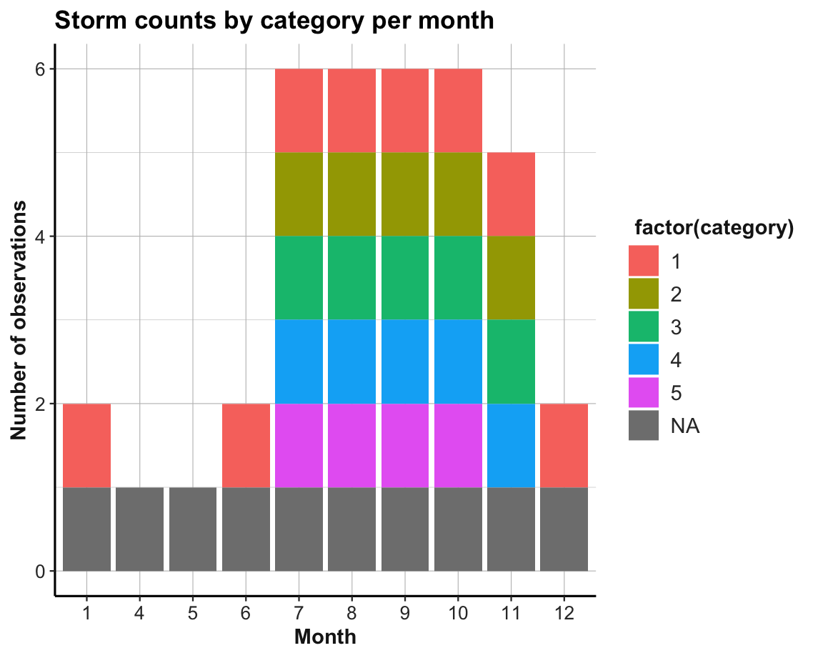

Figure 13.3: Misleading plot version: All storm category counts appear to be 0 or 1.

• What’s the problem with it? How can it be fixed?

Solution 2

The problem is that the bar plot counted how often each category-month combination occurs in t_2 (with geom_bar() using its default stat = "count"). Thus, the only two possible counts for each combination of storm category and month are 0 (i.e., absence of a cell value) and 1 (i.e., presence of a cell value).

Here are two possible corrections:

1. Use t_2 data, but geom_bar() using y = n and stat = "identity":

ggplot(t_2, aes(x = factor(month))) +
  geom_bar(aes(y = n, fill = category), stat = "identity") +
  labs(title = "Storm counts per month", 
       x = "Month", y = "Count of observations") + 
  theme_ds4psy()

2. Use the raw data of st and geom_bar() with default settings (i.e., stat = "count"):

ggplot(st, aes(x = factor(month))) +
  geom_bar(aes(fill = category)) +
  labs(title = "Storm counts per month", 
       x = "Month", y = "Count of observations") + 
  theme_ds4psy()

Both corrections are quite different, but result in the same visualization:

Figure 13.4: Corrected version showing the frequency count of each storm category per month.

Exercise 3: Names of re-occuring storms

1. Identify all storms in st that were observed in more than one year.

2. There are two ways in which a storm name can appear in more than one year:

• A single storm may occur in multiple years (e.g., from December to January)
• A storm name is used repeatedly (i.e., to name different storms in different years)

Check how often each of these cases occurs.

Solution 3

ad 1.: Grouping by the name and year variables, we first count the number of times a storm occurs per year. We then group by name to count storms occurring in more than one year.

st %>% 
  select(name, year) %>%
  group_by(name, year) %>%
  count() %>%
  # select(name, year) %>%
  group_by(name) %>%
  count() %>%
  filter(n > 1) %>%
  head() 

#> # A tibble: 6 × 2
#> # Groups:   name [6]
#>   name        n
#>   <chr>   <int>
#> 1 Alberto     7
#> 2 Alex        4
#> 3 Allison     3
#> 4 Ana         7
#> 5 Andrew      2
#> 6 Arthur      7

  # tail()

Verify these results for some storms:

• Does “Alberto” really occur in 6 different years?

st %>% 
  filter(name == "Alberto") %>%
  group_by(name, year) %>%
  count()
#> # A tibble: 7 × 3
#> # Groups:   name, year [7]
#>   name     year     n
#>   <chr>   <dbl> <int>
#> 1 Alberto  1982    17
#> 2 Alberto  1988    11
#> 3 Alberto  1994    32
#> 4 Alberto  2000    79
#> 5 Alberto  2006    18
#> 6 Alberto  2012    13
#> # … with 1 more row
#> # ℹ Use `print(n = ...)` to see more rows

• Does “Ana” really occur in 7 different years?

st %>% 
  filter(name == "Ana") %>%
  group_by(name, year) %>%
  count()
#> # A tibble: 7 × 3
#> # Groups:   name, year [7]
#>   name   year     n
#>   <chr> <dbl> <int>
#> 1 Ana    1979    19
#> 2 Ana    1985    14
#> 3 Ana    1991    12
#> 4 Ana    1997    15
#> 5 Ana    2003    13
#> 6 Ana    2009    15
#> # … with 1 more row
#> # ℹ Use `print(n = ...)` to see more rows

• Does “Zeta” really occur in 3 different years?

st %>% 
  filter(name == "Zeta") %>%
  group_by(name, year) %>%
  count()
#> # A tibble: 3 × 3
#> # Groups:   name, year [3]
#>   name   year     n
#>   <chr> <dbl> <int>
#> 1 Zeta   2005     8
#> 2 Zeta   2006    23
#> 3 Zeta   2020    23

This concludes our summary of essential dplyr functions (Wickham, François, et al., 2023). To sum up:

Summary: Key dplyr functions (Wickham, François, et al., 2023)

1. arrange() sorts cases (rows);
2. filter() and slice() select cases (rows) by logical conditions;
3. select() selects and reorders variables (columns);
4. mutate() and transmute() compute new variables (columns) out of existing ones;
5. summarise() collapses multiple values of a variable (rows of a column) to a single one;
   
6. group_by() changes the unit of aggregation (in combination with mutate() and summarise()).

+++ here now +++

• remove parts on tidyr (keep in new tidy chapter)
• add new section in tidy chapter on conceptual distinction (messy/tidy)

Overall, combining dplyr functions into pipes provides very flexible and powerful tools for transforming (i.e., reshaping and reducing) data. Next, we will encounter additional functions for data transformation from the tidyr package (in Chapter 14). Whereas many of the dplyr pipes of this chapter reduced our data (e.g., when filtering, selecting, or summarizing variables), the primary purpose of tidyr functions is to re-shape data tables into “tidy” data.

13.4 Conclusion

13.4.1 Summary

This chapter first introduced the pipe operator of magrittr (Bache & Wickham, 2022) and a range of functions for transforming data from dplyr (Wickham, François, et al., 2023) package, which is a key pillar of the tidyverse (Wickham et al., 2019).

and tidyr (Wickham & Girlich, 2024).

So what is the difference between dplyr and tidyr? If we view the functions of both packages as tools, the boundary between both packages is pretty arbitrary: Both packages provide functions for manipulating tables of data.

When reconsidering our distinction between transformations that reduce or reshape data (from Section 13.1), we see that tidyr mostly deals with reshaping data, whereas dplyr mostly allows on-the-fly data reductions (e.g., selections and summaries). In terms of the tasks addressed, the dplyr functions mainly serve to explicate and understand data contained in a table, whereas the tidyr functions aim to clean up data by reshaping it. In practice, most dplyr pipes reduce a complex dataset to answer a specific question. By contrast, the output of tidyr pipes typically serves as an input to a more elaborate data analysis. However, dplyr also provides functions for joining tables and tidyr can be used to select, separate, or unite variables. Thus, the functionalities of both packages are similar enough to think of them as two complementary tools out of a larger toolbox for manipulating data tables — which is why they are both part of the larger collection of packages provided by the tidyverse (Wickham et al., 2019).

Summary: Data transformation reshapes or reduces data.

The magrittr pipe operator %>% turns nested expressions into sequential expressions (Bache & Wickham, 2022).

Key dplyr functions (Wickham, François, et al., 2023) include:

1. arrange() sorts cases (rows);
2. filter() and slice() select cases (rows) by logical conditions;
3. select() selects and reorders variables (columns);
4. mutate() and transmute() compute new variables (columns) out of existing ones;
5. summarise() collapses multiple values of a variable (rows of a column) to a single one;
   
6. group_by() changes the unit of aggregation (in combination with mutate() and summarise()).

13.4.2 Resources

Here are some pointers to related articles, cheatsheets, and additional links:

On pipes

For details on and the differences between the magrittr pipe operator %>% and R’s native pipe operator |>, see

• New features in R 4.1.0 (by Russ Hyde, 2021-05-17)

• The new R pipe (by Elio Campitelli, 2021-05-25)

On dplyr

• See the cheatsheet on transforming data with dplyr from Posit cheatsheets:

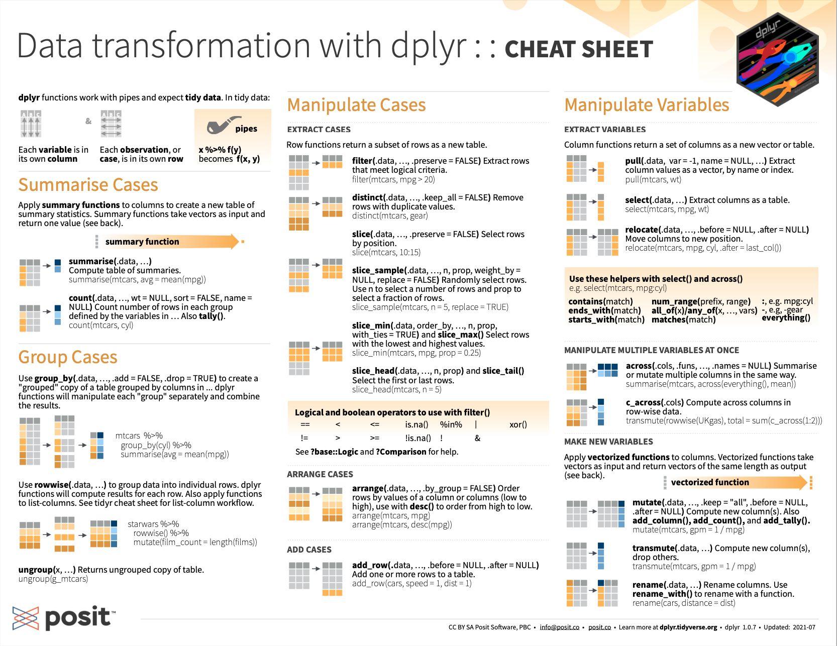
Figure 13.5: Data transformation with dplyr from Posit cheatsheets.

• Introduction on dplyr and pipes: The basics (by Sean C. Anderson, 2014-09-13)

13.4.3 Preview

Having learned how to create data transformation pipes by magrittr and dplyr, the next Chapter 14) on tidying data will expand these skills by adding tools from the tidyr package.

13.5 Exercises

The following exercises on transforming data with the dplyr package (Wickham, François, et al., 2023) are based on Chapter 3: Transforming data of the ds4psy book (Neth, 2023a):

13.5.1 Reshaping vs. reducing data

Exercise 1

13.5.2 Star and R wars

Exercise 2

13.5.3 Sleeping mammals

Exercise 3

13.5.4 Revisiting positive psychology

Exercise 5

13.5.5 Surviving the Titanic

Exercise 6