2 R basics

This chapter provides a very brief introduction to R (R Core Team, 2024), which is a popular language and free software environment for statistical computing and graphics. More specifically, this chapter covers essential concepts and commands of base R, which essentially is what we get when we install R without any additional packages.

Important concepts and contents of this chapter include:

• R objects as data vs. functions;
• creating and changing R objects (by assignment);
• different types of data (e.g., Boolean values of type logical, numbers of type integer or double, and text of type character);
• exploring functions and their arguments.

An important constraint of this chapter is that we mostly ignore the shape of data objects. But as any data object comes in some shape, we will use vectors as our first data structure to explore. This allows us to introduce key concepts of R like subsetting (aka. indexing or filtering) and recycling.

Overall, a firm grasp of these basic notions (i.e., objects, data types vs. shapes, vectors, indexing, and recycling) is fundamental to understanding R. In Chapter 3 on Data structures, we will encounter additional data structures (e.g., matrices, lists, tables, and data frames) and realize that what we have learned for vectors can be transferred to them.

Preparation

This chapter assumes that you have access to a working version of R, the RStudio IDE, and the R packages of the tidyverse (Wickham, 2023b) and ds4psy (Neth, 2023b). Its contents are mostly based on

• Chapter 1: Basic R concepts and commands (Neth, 2023a)

However, the first chapter of the ds4psy book also introduces data structures beyond vectors, which we will cover in a separate Chapter 3.

Preflections

Before reading, please take some time to reflect upon the following questions:

• What is being manipulated by computer code?

• How can a data object be changed by code?

• Which types of data can we distinguish?

• In which order is computer code evaluated?

• Which windows in the RStudio IDE allow interacting with R?

Please note: The purpose of these questions to help you adopt various perspectives and a reflective state of mind. Do no worry if they seem difficult or obscure at this point. Hopefully, their answers will become clearer by the end of the chapter.

2.1 Introduction

Mastering R (or any other programming language) essentially consists in solving two inter-related tasks:

1. Defining various types of data as objects (Section 2.2).

2. Manipulating these objects by using functions (Section 2.4).

This chapter introduces both of these tasks. Later, we will see that analyzing data often involves creating and manipulating additional data structures (Chapter 3) and that the activity of programming usually involves creating our own processes (Chapters 4 and 6) and functions (Chapter 5). But before we can address more advanced issues, we need to grasp the difference between between “data” (as some object that represents particular types of information) vs. “functions” (as operators that process and transform information).

The main type of object used in R for representing data is a vector. Vectors come in different data types and shapes and have some special properties that we need to know in order to use them in a productive fashion. As we will see, manipulating vectors by applying functions to them allows for quite a bit of data analysis — and all the rest are details and extensions…

2.1.1 Contents

This chapter introduces basic concepts and essential R commands. It rests on the distinction between “data objects” and “functions” and introduces “vectors” as the key data structure of R. Vectors come in different data “types” (e.g., character, numeric, logical) and “shapes” (short or long), and — like any other data object — are manipulated by suitable “functions”. Key concepts for working with vectors in R are “assignment”, “recycling”, and “filtering” (aka. “indexing” or “subsetting”). Again, the limitation of this chapter (in contrast to Chapter 3) is that it does not cover data structures beyond vectors.

2.1.2 Data and tools

This chapter only uses base R functions and snippets of example data that we will generate along the way. Some examples are using functions provided by the ds4psy package (Neth, 2023b).

2.2 Defining R objects

To understand computations in R, two slogans are helpful:
- Everything that exists is an object.
- Everything that happens is a function call.

John Chambers

Everything that exists in R must be represented somehow. A generic term for something that we know not much about is an object. In R, we can distinguish between two main types of objects:

1. data objects are typically passive containers for values (e.g., numbers, truth values, or strings of text), whereas

2. function objects are active elements or tools: They do things with data.

When considering any data object, we can always ask two questions:

1. What type of data is it?

2. In what shape is the data represented?

Particular combinations of data types and shapes are known as data structures. Distinguishing between different data types (in Section 2.2.2) and data structures (in Section 3.2) is an important goal of the current chapter and Chapter @(struc). To illustrate the data types and data structures that are available in R, we first need to explain how to define corresponding data objects (in Section 2.2.1. This will involve “doing something” with data, i.e., using functions (in Section 2.4).

2.2.1 Data objects

When using R, we typically create data objects that store the information that we care about (e.g., some data file). To achieve our goals (e.g., understand or reveal some new aspect of the data), we use or design functions as tools for manipulating and changing data (e.g., inputs) to create new data (e.g., outputs).

Creating and changing objects by assignment

Objects are created or changed by assignment using the <- operator and the following structure:

obj_name <- value

Here are definitions of four different types of objects:

lg <- TRUE
n1 <- 1
n2 <- 2L
cr <- "hi"

To determine the type of these objects, we can evaluate the typeof() function on each of them:

typeof(lg)
#> [1] "logical"
typeof(n1)
#> [1] "double"
typeof(n2)
#> [1] "integer"
typeof(cr)
#> [1] "character"

To do something with these objects, we can apply other functions to them:

!lg        # negate a logical value
#> [1] FALSE
n1         # print an object's current value
#> [1] 1
n1 + n2    # add 2 numeric objects
#> [1] 3
nchar(cr)  # number of characters
#> [1] 2

To change an object, we need to assign something else to it:

n1 <- 8  # change by re-assignment 
n1
#> [1] 8
n1 + n2
#> [1] 10

Note that the last two code chunks contained the lines n1 and n1 + n2 twice, but yielded different results. The reason is that n1 was initially assigned to 1, but then changed (or rather was re-assigned) to 8. This implies that R needs to keep track of all our current variable bindings. This is done in R’s so-called environment (see the “Environment” tab of the RStudio IDE). Although the reality is a bit more complicated (due to a hierarchical structure of multiple layers), we can think of the environment as a collection of all current objects and their assigned values. When a new object is assigned, it is created and added to the environment. When an existing object is re-assigned, its value in the environment changes to the new one.

As R’s current environment is an important feature of R, here is another example: Changing an object by re-assigning it creates multiple “generations” of an object. In the following code, the logical object lg refers to two different truth values at different times:

lg         # assigned to TRUE (above)
#> [1] TRUE
lg <- !lg  # change by re-assignment  
lg         # assigned to FALSE (now) 
#> [1] FALSE

Here, the value of the logical object lg changed from TRUE to FALSE by the assignment lg <- !lg. As this assignment negates the current value of an object, the value of lg on the left of the assignment operator <- differs from the value of lg on its right. When explicated in such detail, this sounds a bit like magic, but is merely the combined function of combining the ! and <- operators. Importantly, whenever an object (e.g., lg) is re-assigned, its previous value(s) are lost, unless they have been assigned to (or stored as) a different object.

Naming objects

Naming objects (both data objects and functions) is an art in itself. A good general recommendation is to always aim for consistency and clarity. This may sound trivial, but if you ever tried to understand someone else’s code — including your own from a while ago — it is astonishing how hard it actually is.

Here are some generic recommendations (some of which may be personal preferences):

• Always aim for short but clear and descriptive names:
  • data objects can be abstract (e.g., abc, t_1, v_output) or short words or abbreviations (e.g., data, cur_df),
  • functions should be verbs (like print()) or composita (e.g., plot_bar(), write_data()).

• Honor existing conventions (e.g., using v for vectors, i and j for indices, x and y for coordinates, n or N for sample or population sizes, …).

• Create new conventions when this promotes consistency (e.g., giving objects that belong together similar names, or calling all functions that plot something with plot_...(), that compute something with comp_...(), etc.).

• Use only lowercase letters and numbers for names (as they are easy to type — and absolutely avoid all special characters, as they may not exist or look very different on other people’s computers),

• Use snake_case for combined names, rather than camelCase, and — perhaps most importantly —

• Break any of those rules if there are good (i.e., justifiable) reasons for this.

2.2.2 Data types

For any data object, we distinguish between its shape and its type. The shape of an object mostly depends on its structure. As this chapter uses only a single data structure (i.e., vectors), we will address issues of data shape later (in Chapter 3 on Data structures).

Here, we focus on data types (which are also described as data modes in R). Throughout this book, we will work with the following data types:

1. logical values (aka. Boolean values, of type logical)
2. numbers (of type integer or double)
3. text or string data (of type character)
4. dates and times (with various data types)

We already defined objects of type “integer”, “double”, “character” and “logical” above. To check the type of a data object, two elementary functions that can be applied to any R object are typeof() and mode():

typeof(TRUE)
#> [1] "logical"
typeof(10L)
#> [1] "integer"
typeof(10)
#> [1] "double"
typeof("oops")
#> [1] "character"

mode(TRUE)
#> [1] "logical"
mode(10L)
#> [1] "numeric"
mode(10)
#> [1] "numeric"
mode("oops")
#> [1] "character"

Note that R distinguishes between two numeric data types (integer and double), but both of them are of numeric mode.

If we want to check objects for having a particular data type, the following functions allow asking more specific questions:

is.character(TRUE)
#> [1] FALSE
is.double(10L)
#> [1] FALSE
is.integer(10)
#> [1] FALSE
is.numeric("oops")
#> [1] FALSE

To check the shape of a data object, two basic functions that can be applied to many R objects are length() and str():

length(FALSE)
#> [1] 1
length(100L)
#> [1] 1
length(123)
#> [1] 1
length("hey")
#> [1] 1

str(FALSE)
#>  logi FALSE
str(100L)
#>  int 100
str(123)
#>  num 123
str("hey")
#>  chr "hey"

The length() function actually describes a basic property of the most fundamental data structure in R: Atomic vectors. Vectors with a length of 1 are known as scalar objects.

As the objects checked here are pretty simple (i.e., they all are scalars), the results of these functions are pretty boring. But as we move on to more complex data structures, we will learn more ways of checking object shapes and encounter richer data structures.

At this point, it is good to note that even data objects that may look more complicated can internally be simple objects:

In the following sections, we explore each of the four main data types by applying typical functions to corresponding data objects.

Logicals

The simplest data types are logical values (aka. Boolean values).
Logical values exist in exactly two varieties: TRUE and FALSE.

A <- TRUE
B <- FALSE

It is possible in R to abbreviate TRUE and FALSE by T and F. However, as T and F are non-protected names and can also be set to other values, these abbreviations should be avoided.

By combining logical values with logical operators, we can create more complex logical expressions:

!A        # negation (NOT)
#> [1] FALSE
A & B     # conjunction (AND)
#> [1] FALSE
A | B     # disjunction (OR)
#> [1] TRUE
A == !!A  # equality (+ double negation)
#> [1] TRUE

The definition of these operators follows standard propositional logic (see Wikipedia: Logical connective for details):

• Negation (NOT): !A reverses/swaps the truth value of A
• Conjunction (AND): A & B is TRUE iff (if and only if) A and B are both TRUE
• Disjunction (OR): A | B is TRUE iff A or B or both are TRUE
• Equality: A == B is TRUE iff A and B are both TRUE or both FALSE

The result of evaluating any logical expression is a logical value (i.e., TRUE or FALSE).

By combining logical objects and operators, we can express quite fancy statements of propositional logic. For instance, the following statements verify the validity of De Morgan’s Laws (e.g., on Wikipedia) in R:

A <- TRUE   # either TRUE or FALSE.
B <- FALSE  # either TRUE or FALSE.

# (1) not (A or B) = not A and not B:
!(A | B) == (!A & !B)

# (2) not (A and B) = not A or not B:
!(A & B) == (!A | !B)

Irrespective of the truth value of A and B, the statements (1) and (2) are always TRUE.

When doubling the logical operators | or &, R carries out their evaluation sequentially (from left to right) and returns a logical value as soon as possible (i.e., skipping any remaining checks). Thus,

TRUE  || stop("error")  # --> TRUE
FALSE || stop("error")  # --> error
TRUE  && stop("error")  # --> error
FALSE && stop("error")  # --> FALSE

A noteworthy feature of R is that logical values are interpreted as numbers (introduced as our next data type) when the context suggests this interpretation. In these cases, any value of TRUE is interpreted as the number 1 and any value of FALSE is interpreted as the number 0. The following examples illustrate what happens when logical values appear in calculations:

TRUE + FALSE
#> [1] 1
TRUE - FALSE + TRUE
#> [1] 2
3 * TRUE - 11 * FALSE/7
#> [1] 3

The same interpretation of truth values is made when applying arithmetic functions to (vectors of) truth values:

sum(c(TRUE, FALSE, TRUE))
#> [1] 2
mean(c(TRUE, FALSE, FALSE))
#> [1] 0.3333333

Calculating with logical values may seem a bit strange at first, but provides a useful bridge between logical and numeric data types.

Practice: Working with logical numbers

Assume a confused person had made the following assignments:¹⁶

T <- FALSE
F <- TRUE

• Predict, evaluate, and explain the results of the following expressions:

!!!T
T == FALSE
F != FALSE
T | FALSE
T || TRUE
T + TRUE - F

Numbers

Numbers can be represented and entered into R in a variety of ways. In most cases, they are either entered using the decimal notation, as the result of computations, or in scientific notation (using the e\(x\) notation to indicate the \(x\)-th power of 10). By default, R represents all numbers as data of type double.

Here are different ways of entering the number 3.14 and then testing for its type:

typeof(3.14)          # decimal
#> [1] "double"
typeof(314/100)       # ratio
#> [1] "double"
typeof(3.14e0)        # scientific notation
#> [1] "double"
typeof(round(pi, 2))  # a built-in constant
#> [1] "double"

If we specifically want to represent a number as an integer, it must not contain a fractional part and be followed by L (reminiscent of the “Long” data type in C):

typeof(123)
#> [1] "double"
typeof(123L)
#> [1] "integer"

Note that entering a decimal number with an added L (e.g., 3.14L) would return the decimal number with a warning, as integers cannot contain fractional values.

Three special numeric values are infinity (positive Inf and negative -Inf) and non-numbers (NaN):

 1/0  # positive infinity
#> [1] Inf
-1/0  # negative infinity
#> [1] -Inf
 0/0  # not defined
#> [1] NaN

In these examples, we use the / operator to indicate a fraction or “division by” operation. The results computed and printed by R conform to our standard axioms of arithmetic.

Note that NaN is different from a missing number (denoted in R as NA) and that the data type of these special numbers is still double:

typeof(1/0)
#> [1] "double"
typeof(0/0)
#> [1] "double"

Numbers are primarily useful for calculating other numbers from them. This is either done by applying numeric functions, but also by applying arithmetic operators to numeric objects.

To gain further insights on numeric objects, we usually apply numeric functions to them. In the next example, the R object nums is defined as a vector nums, which contains five numbers (see more on vectors below).

• Doing statistics in R essentially means to apply statistical functions to data objects. The following basic functions examine and describe a numeric data object nums:

# Define a numeric vector:
nums <- c(-10, 0, 2, 4, 6)

# basic functions:
length(nums) # nr. of elements
#> [1] 5
min(nums)    # minimum 
#> [1] -10
max(nums)    # maximum
#> [1] 6
range(nums)  # min - max
#> [1] -10   6

# aggregation functions:
sum(nums)   # sum
#> [1] 2
mean(nums)  # mean
#> [1] 0.4
var(nums)   # variance
#> [1] 38.8
sd(nums)    # standard deviation
#> [1] 6.228965

• Computing with numbers requires arithmetic operations (e.g., addition, subtraction, etc.). Here are examples of the the most common arithmetic operators:

x <- 5
y <- 2

+ x      # keeping sign 
#> [1] 5
- y      # reversing sign
#> [1] -2
x + y    # addition
#> [1] 7
x - y    # subtraction
#> [1] 3
x * y    # multiplication
#> [1] 10
x / y    # division
#> [1] 2.5
x ^ y    # exponentiation
#> [1] 25
x %/% y  # integer division
#> [1] 2
x %% y   # remainder of integer division (x mod y)
#> [1] 1

• When an arithmetic expression contains more than one operator, the issue of operator precedence arises. When combining different operators, R uses the precedence rules of the so-called “BEDMAS” order:

• Brackets (),

• Exponents ^,

• Division / and Multiplication *,

• Addition + and Subtraction -

1 / 2 * 3    # left to right
#> [1] 1.5
1 + 2 * 3    # precedence: */ before +-
#> [1] 7
(1 + 2) * 3  # parentheses change precedence
#> [1] 9

2^1/2   == 1
#> [1] TRUE
2^(1/2) == sqrt(2)
#> [1] TRUE

Evaluating ?Syntax provides the full list of rules for operator precedence. However, using parentheses to structure longer (arithmetic or logical) expressions always increases transparency.

Numbers can also be compared to other numbers. When comparing numbers (i.e., applying comparison operators to them), we get logical values (i.e., scalars of type “logical” that are either TRUE or FALSE).

• For instance, each of the following comparisons of numeric values yields a logical object (i.e., either TRUE or FALSE) as its result:

2 > 1   # larger than
#> [1] TRUE
2 >= 2  # larger than or equal to
#> [1] TRUE
2 < 1   # smaller than
#> [1] FALSE
2 <= 1  # smaller than or equal to
#> [1] FALSE

The operator == tests for the equality of objects, whereas != tests for inequality (or non-equality):

1 == 1  # == ... equality
#> [1] TRUE
1 != 1  # != ... inequality 
#> [1] FALSE

A common source of errors in R is that novices tend to confuse = with ==. As the single equal symbol = is an alternative assignment operator <-, trying to use it as a logical operator yields unexpected results (“assignment errors”). But using the == operator for testing the equality of two objects can also be error-prone when dealing with non-trivial objects (e.g., computed or named objects). For example, when squaring the square-root of x, we expect to obtain the original x:

# A mathematical puzzle:
x <- sqrt(2)
x^2 == 2  # mathematically TRUE, but: 
#> [1] FALSE

The reason for this surprising violation of a mathematical truth lies in the representation of numbers. In principle, the squared square root of x is equal to x (assuming standard mathematical axioms). In practice, the represented results of numerical operations show tiny deviations from their theoretical values:

# Reason:
x^2 - 2   # tiny numeric difference
#> [1] 4.440892e-16

As computers store (real) numbers as approximations (so-called floating point numbers), x == y can evaluate to FALSE even the values of x and y should be equal. The solution for checking for the equality of numbers, consists in using functions that allow for minimal tolerances (that must be low enough to not matter for the task at hand). One such function is all.equal():

all.equal(x^2, 2)
#> [1] TRUE

The base R function all.equal() accepts additional arguments that determine whether names or other attributes are being considered. As checking for equality is a common task, many R packages provide corresponding functions (e.g., see near() of dplyr, or num_equal() and is_equal() of ds4psy).

Practice: Working with numbers

Assume the following definitions:

x <- 2L
y <- 3^{1/x}
z <- y^x

1. What is the data type, value, and shape of x, y, and z?

2. What is the result of x + x / x? Why?

3. What is the result of y^x != z? Why?

4. What is the result of sqrt(x)^x == z - 1? Why?

#> [1] "integer"
#> [1] "double"
#> [1] 3
#> [1] FALSE
#> [1] TRUE
#> [1] TRUE
#> [1] TRUE
#> [1] FALSE
#> [1] TRUE
#> [1] TRUE
#> [1] TRUE

Characters

Text data (also called “strings”) is represented as data of type character. To distinguish character objects from the names of other R objects, they need to be surrounded by double quotes (as in “hello”) or single quotes (as in ‘bye’). Special characters (that have a special meaning in R) are escaped with a backslash (e.g., \;, see ?Quotes for details).

The length of a word w is not determined by length(w), but by a special function nchar() (for “number of characters”). The following proves that word is a four-letter word:

nchar("word")
#> [1] 4

Alphabetical characters come in two varieties: lowercase (e.g., a, b, c) and uppercase (e.g., A, B, C). R comes with two corresponding built-in constants:

letters
#>  [1] "a" "b" "c" "d" "e" "f" "g" "h" "i" "j" "k" "l" "m" "n" "o" "p" "q" "r" "s"
#> [20] "t" "u" "v" "w" "x" "y" "z"
LETTERS
#>  [1] "A" "B" "C" "D" "E" "F" "G" "H" "I" "J" "K" "L" "M" "N" "O" "P" "Q" "R" "S"
#> [20] "T" "U" "V" "W" "X" "Y" "Z"

that provide vectors containing the 26 characters of the Western alphabet (in lowercase vs. uppercase letters, respectively) and special functions that evaluate or change objects of type of character:

slogan <- "Make America green again."
nchar(slogan)
#> [1] 25
toupper(slogan)
#> [1] "MAKE AMERICA GREEN AGAIN."
tolower(slogan)
#> [1] "make america green again."

In terms of representation, the difference between "A" and "a" is not one of data type. They are both characters (i.e., objects of type “character”), but different ones.

The most prominent function for working with character data is paste(), which does what it says:

paste("This", "is", "a", "sentence.")
#> [1] "This is a sentence."
paste("This", "is", "a", "sentence.", sep = " - ")
#> [1] "This - is - a - sentence."

As there are many different scenarios for pasting individual character objects into larger ones, the paste() function comes with interesting options and variants. As Chapter 17 is devoted to text data, we do not cover them here.

Practice: Representing characters

Assume the following assignments of R objects:

x <- "a"
y <- 2
X <- "A"
Y <- "B"
Z <- "AB"

1. It which sense(s) are x and y similar and different?
2. It which sense(s) are x and X similar and different?
3. It which sense(s) are X, Y, and Z similar and different?

The terms “similar and different” can refer to the data type and shape of representations or their represented meanings. (We can answer these questions analytically, or use R functions to help us out.)

4. What is the result of paste(X, "+", Y, "=", Z)? Why?

5. What is the result of length("word")? Why?

#> [1] TRUE
#> [1] "character"
#> [1] "double"
#> [1] TRUE
#> [1] TRUE
#> [1] TRUE
#> [1] TRUE
#> [1] TRUE
#> [1] TRUE
#> [1] TRUE
#> [1] "A + B = AB"
#> [1] 1

Dates and times

Dates and times are more complicated data types — not because they are complicated per se, but because their definition and interpretation needs to account for a lot of context and conventions, plus some irregularities. At this early point in our R careers, we only need to know that such data types exist. Two particular functions allow to illustrate them and are quite useful, as they provide the current date and time:

Sys.Date()
#> [1] "2022-09-07"
Sys.time()
#> [1] "2022-09-07 20:01:34 CEST"

Note the data type (and mode) of both:

typeof(Sys.Date())
#> [1] "double"
mode(Sys.Date())
#> [1] "numeric"
unclass(Sys.Date())  # show internal representation
#> [1] 19242

typeof(Sys.time())
#> [1] "double"
mode(Sys.time())
#> [1] "numeric"
unclass(Sys.time())  # show internal representation
#> [1] 1662573694

Thus, R internally stores dates and times as numbers (of type “double”), but then interprets them to print them in a format facilitates our interpretation of them. Note that this format is subject to many conventions and idiosyncrasies (e.g., regarding the arrangement of elements and local time zones). Chapter 18 is devoted to working with time data in R.

Missing values

The final concept considered here is not a type of data, but a type of value. What happens when we do not know the value of a variable? In R, a lacking or missing value is represented by NA, which stands for not available, not applicable, or missing value:

# Assign a missing value:
ms <- NA
ms
#> [1] NA

# Data type?
typeof(ms)
#> [1] "logical"
mode(ms)
#> [1] "logical"

By default, NA is of a logical data type, but other data types have their own type of NA value: NA_integer_ (for a missing integer), NA_real_ (for a missing double), and NA_character_ (for a missing character). But as the data types of NA values are flexibly changed into each other when necessary, we can usually ignore this distinction.

As missing values are quite common in real-world data, we need to know how to deal with them. The function is.na() allows us to test for a missing value:

is.na(12)
#> [1] FALSE
is.na(NA)
#> [1] TRUE

In R, NA values are typically “addictive” in the sense of creating more NA values when applying functions to them:

NA + 1
#> [1] NA
sum(1, 2, NA, 4)
#> [1] NA

but many functions have ways of instructing R to ignore missing values. For instance, many numeric functions accept a logical argument na.rm that remove any NA values:

sum(1, 2, NA, 4, na.rm = TRUE)
#> [1] 7

Note that combining NA values with logical values can have unexpected consequences:

NA & FALSE
#> [1] FALSE
NA & TRUE
#> [1] NA
NA | FALSE
#> [1] NA
NA | TRUE
#> [1] TRUE

To make sense of these results, we can imagine that NA lies between FALSE and TRUE.

Practice: Missing values

Predict, evaluate, and explain the result of the following expressions:

is.na("NA")
is.na(some_undefined_object)
NA || FALSE
NA && FALSE
2 * NA
2 * NA == NA / 2

2.3 Vectors

We mentioned above that every data object can be described by its shape and its type. Whereas we addressed the issue of data types (and the related term of modes, see Section 2.2.2), we have not yet discussed the shape of data objects.

All objects defined so far all shared the same shape: The were vectors that only contained a single element. In R, vectors of length 1 are known as scalars.

Vectors are by far the most common and most important data structure in R. Essentially, a vector v is an ordered sequence of elements with three common properties:

1. the type of its elements (available by typeof(v));
   
2. its length (available by length(v));
3. optional attributes or meta-data (tested by attributes(v)).

More specifically, R uses two types of vectors:

• in atomic vectors, all elements are of the same data type;
  
• in lists, different elements can have different data types.

The vast majority of vectors we will encounter are atomic vectors (i.e., all elements have the same data type), but lists are often used in R for storing a variety of data types in a common object (e.g., in statistical analyses). It is important to understand that the term “atomic” in “atomic vectors” refers to the type of the vector, rather than its shape or length: Atomic vectors can contain one or more elements of some data type (i.e., they can have different lengths), but cannot contain multiple data types.

How can we create new vectors? We already encountered a basic way of creating a vector above: Creating a new data object by assigning a value to an object name (using the <- operator). As any scalar object already is a vector (of length 1), we actually are asking: How can we combine objects (or short vectors) into longer vectors?

The main way of creating a vector is by using the c() function (think chain, combine, or concatenate) on a number of objects:

# Create vectors:
v_lg <- c(TRUE, FALSE)   # logical vector
v_n1 <- c(1, pi, 4.5)    # numeric vector (double)
v_n2 <- c(2L, 4L, 6L)    # numeric vector (integer)
v_cr <- c("hi", "Hallo", "salut")  # character vector

The vectors defined by combining existing vectors with the c() function typically are longer vectors than their constituents.

Whenever encountering a new vector, a typical thing to do is testing for its type and its length:

# type:
typeof(v_n1)
#> [1] "double"
typeof(v_cr)
#> [1] "character"
# length: 
length(v_lg)
#> [1] 2
length(v_n2)
#> [1] 3

Beyond these elementary functions, the majority of functions in R can be applied to vectors. However, most functions require a particular data type to work properly. For instance, a common operation that changes an existing vector consists in sorting vectors, which is achieved by the sort() function. An argument decreasing is set to FALSE by default, but can be set to TRUE if sorting in decreasing order is desired:

x <- c(4, 6, 2)

sort(x)
#> [1] 2 4 6
sort(x, decreasing = TRUE)
#> [1] 6 4 2

What happens when we apply sort() to other data types?

y <- c(TRUE, FALSE, TRUE, FALSE)
sort(y)
#> [1] FALSE FALSE  TRUE  TRUE

z <- c("A", "N", "T")
sort(z, decreasing = TRUE)
#> [1] "T" "N" "A"

This shows that generic R functions like sort() often work with multiple data types. However, many functions simply require specific data types and would not work with others. For instance, as most mathematical functions require numeric objects to work, the following would create an error:

sum("A", "B", "C")  # would yield an error

However, remember that vectors of logical values can be interpreted as numbers (FALSE as 0 and TRUE as 1):

v_lg2 <- c(FALSE, TRUE, FALSE)
v_nm2 <- c(4, 5)

c(v_lg2, v_nm2)
#> [1] 0 1 0 4 5
mean(v_lg2)
#> [1] 0.3333333

As attributes are optional, most (atomic) vectors have no attributes:

v_n2
#> [1] 2 3 5
attributes(v_n2)
#> NULL

The most common attribute of a vector \(v\) are the names of its elements, which can be set or retrieved by names(v):

# Setting names:
names(v_n2) <- c("A", "B", "C")
names(v_cr) <- c("en", "de", "fr")

# Getting names:
names(v_n2)
#> [1] "A" "B" "C"

Other attributes can be defined as name-value pairs using attr(v, name) <- value) and inspected by attributes(), str() or structure():

# Adding attributes:
attr(v_cr, "my_dictionary") <- "Words to greet people"

# Viewing attributes:
attributes(v_n2)
#> $names
#> [1] "A" "B" "C"
attributes(v_cr)
#> $names
#> [1] "en" "de" "fr"
#> 
#> $my_dictionary
#> [1] "Words to greet people"

# Inspecting a vector's structure: 
str(v_cr)
#>  Named chr [1:3] "hi" "Hallo" "salut"
#>  - attr(*, "names")= chr [1:3] "en" "de" "fr"
#>  - attr(*, "my_dictionary")= chr "Words to greet people"
structure(v_cr)
#>      en      de      fr 
#>    "hi" "Hallo" "salut" 
#> attr(,"my_dictionary")
#> [1] "Words to greet people"

There exists an is.vector() function in R, but it does not only test if an object is a vector. Instead, it returns TRUE only if the object is a vector with no attributes other than names.

To test if an object v actually is a vector, we can use is.atomic(v) | is.list(v) (i.e., test if it is an atomic vector or a list) or use an auxiliary function by another R package (e.g., is_vect() of ds4psy or is_vector() of purrr):

# (1) A vector with only names:
is.vector(v_n2)
#> [1] TRUE

# (2) A vector with additional attributes:
is.vector(v_cr)
#> [1] FALSE

# but:
is.atomic(v_cr)
#> [1] TRUE
ds4psy::is_vect(v_cr)
#> [1] TRUE
purrr::is_vector(v_cr)
#> [1] TRUE

2.3.1 Creating vectors

We have already seen that using the assignment operator <- creates new data objects and that the c() function combines (or concatenates) objects into vectors. When the objects being combined are already stored as vectors, we are actually creating longer vectors out of shorter ones:

# Combining scalar objects and vectors (into longer vectors): 
v1 <- 1          # same as v1 <- c(1)
v2 <- c(2, 3)

v3 <- c(v1, v2, 4)  # but the result is only 1 vector, not 2 or 3: 
v3
#> [1] 1 2 3 4

Note that the new vector v4 is still a vector, rather than some higher-order structure containing other vectors (i.e., c() flattens hierarchical vector structures into vectors).

Coercion of data types

The key limitation of an atomic vector in R is that all its elements share the same data type. This raises the question:

• What happens, when we combine objects of different data types in a vector?

When combining different data types into an atomic vector, they are coerced into a single data type. The result is either a numeric vector (when mixing truth values and numeric objects) or a character vector (when mixing anything with characters):

# Combining different data types:
x <- c(TRUE, 2L, 3.0)  # logical, integer, double
x
#> [1] 1 2 3
typeof(x)
#> [1] "double"

y <- c(TRUE, "two")  # logical, character
y
#> [1] "TRUE" "two"
typeof(y)
#> [1] "character"

z <- c(TRUE, 2, "three")  # logical, numeric, character
z
#> [1] "TRUE"  "2"     "three"
typeof(z)
#> [1] "character"

The R data type "double" allows expressing both logical objects (i.e., TRUE or FALSE as 1 or 0) and numeric data types (integers and doubles as doubles). Similarly, the R data type "character" provides an umbrella data type that allows representing all other data types (e.g., the value of pi as a character object "3.141593"). Importantly, such re-representations of objects in a different data type changes what we can do with them (i.e., which functions we can apply to them). For instance, we can apply the function nchar() to "3.141593", but no longer apply + or round() to them (as "3.141593" is a character object, rather than a number). To interpret and use "3.141593" as a number, we first need to apply as.numeric() to it.

Recycling vectors

When dealing with vectors with different shapes, we can ask:

• What happens, when we apply functions to vectors of different lengths?

As when combining different data types, the vectors are coerced to a common shape. More specifically, the process called recycling repeats the elements of any shorter vector until it matches the length of the longest vector. This works quite intuitively when the elements of the longer vector is a multiple of the shorter vector:

c(2, 4, 6) / 2
#> [1] 1 2 3
c(TRUE, FALSE, TRUE, FALSE) | c(FALSE, TRUE)
#> [1] TRUE TRUE TRUE TRUE
paste0(c("feel", "hurt"), "ing")
#> [1] "feeling" "hurting"

but may require some fiddling (and Warnings) when the shorter vector does not fit neatly into the longer one:

c(10, 15, 20) + c(1, 2)
#> [1] 11 17 21
c(TRUE, FALSE, TRUE, FALSE) & c(FALSE, TRUE, TRUE)
#> [1] FALSE FALSE  TRUE FALSE
paste0(c("cat", "dog", "cow"), c("s", " 2"))
#> [1] "cats"  "dog 2" "cows"

Overall, we can summarize:

• When creating vectors out of different data types, they are coerced into a single type.
• When using vectors of different shapes, they are coerced into a single shape.

Vector creation functions

The c() function is used for combining existing vectors. However, for creating vectors that contain more than just a few elements (i.e., vectors with larger length() values), using the c() function and then typing all vector elements becomes impractical. Useful functions and shortcuts to generate continuous or regular sequences are the colon operator :, and the functions seq() and rep():

• m:n generates a numeric sequence (in steps of \(1\) or \(-1\)) from m to n:

# Colon operator (with by = 1):
s1 <- 0:10
s1
#>  [1]  0  1  2  3  4  5  6  7  8  9 10
s2 <- 10:0
all.equal(s1, rev(s2))
#> [1] TRUE

• seq() generates numeric sequences from an initial number from to a final number to and allows either setting the step-width by or the length of the sequence length.out:

# Sequences with seq():
s3 <- seq(0, 10, 1)  # is short for: 
s3
#>  [1]  0  1  2  3  4  5  6  7  8  9 10
s4 <- seq(from = 0, to = 10, by = 1)
all.equal(s3, s4)
#> [1] TRUE
all.equal(s1, s3)
#> [1] TRUE

# Note: seq() is more flexible:
s5 <- seq(0, 10, by = 2.5)        # set step size
s5
#> [1]  0.0  2.5  5.0  7.5 10.0
s6 <- seq(0, 10, length.out = 5)  # set output length
all.equal(s5, s6)
#> [1] TRUE

• rep() replicates the values provided in its first argument x either times times or each element each times:

# Replicating vectors (with rep):
s7 <- rep(c(0, 1), 3)  # is short for:
s7
#> [1] 0 1 0 1 0 1
s8 <- rep(x = c(0, 1), times = 3)
all.equal(s7, s8)
#> [1] TRUE

# but differs from:
s9 <- rep(x = c(0, 1), each = 3)
s9
#> [1] 0 0 0 1 1 1

Whereas : and seq() create numeric vectors, rep() can be used with other data types:

rep(c(TRUE, FALSE), times = 2)
#> [1]  TRUE FALSE  TRUE FALSE
rep(c("A", "B"), each = 2)
#> [1] "A" "A" "B" "B"

Random sampling from a population

A frequent situation when working with R is that we want a sequence of elements (i.e., a vector) that are randomly drawn from a given population. The sample() function allows drawing a sample of size size from a population x. A logical argument replace specifies whether the sample is to be drawn with or without replacement. Not surprisingly, the population x is provided as a vector of elements and the result of sample() is another vector of length size:

# Sampling vector elements (with sample):
sample(x = 1:3, size = 10, replace = TRUE)
#>  [1] 1 2 1 2 3 1 2 2 2 2
# Note:
# sample(1:3, 10)  
# would yield an error (as replace = FALSE by default). 

# Note:
one_to_ten <- 1:10
sample(one_to_ten, size = 10, replace = FALSE)  # drawing without replacement
#>  [1]  3  5  8  1  6  7  2 10  4  9
sample(one_to_ten, size = 10, replace = TRUE)   # drawing with replacement
#>  [1]  2  4  3  7 10  2  5  3  1  3

As the x argument of sample() accepts non-numeric vectors, we can use the function to generate sequences of random events. For instance, we can use character vectors to sample sequences of letters or words (which can be used to represent random events):

# Random letter/word sequences:
sample(x = c("A", "B", "C"), size = 10, replace = TRUE)
#>  [1] "C" "A" "B" "C" "C" "C" "C" "B" "A" "B"
sample(x = c("he", "she", "is", "good", "lucky", "sad"), size = 5, replace = TRUE)
#> [1] "lucky" "she"   "good"  "is"    "good"

# Binary sample (coin flip): 
coin <- c("H", "T")    # 2 events: Heads or Tails
sample(coin, 5, TRUE)  # is short for: 
#> [1] "T" "H" "T" "T" "H"
sample(x = coin, size = 5, replace = TRUE)    # flip coin 5 times
#> [1] "H" "H" "T" "T" "H"

# Flipping 10.000 coins:
coins_10000 <- sample(x = coin, size = 10000, replace = TRUE)  # flip coin 10.000 times
table(coins_10000)  # overview of 10.000 flips
#> coins_10000
#>    H    T 
#> 5049 4951

Let’s practice what we have learned so far:

2.3.2 Practice

Vectors vs. other data structures

1. Describe the attributes of an atomic vector in R.

2. Here are three R objects x, y and z:

x
#> [1] 123456789
y
#> [1] "TEq"    "EIcF"   "FIY"    "ZEYW"   "lGSE"   "zVPZ"   "utnhW"  "fxMjWy"
#> [9] "iFKq"
z
#> [[1]]
#> [1] TRUE
#> 
#> [[2]]
#> [1] "FIY"    "TEq"    "fxMjWy"
#> 
#> [[3]]
#> [1] 123456789

• Describe these objects in terms of their data types and shapes.
• Which of these objects are atomic?
• In what respects are they similar? How do they differ from each other?

Creating vectors

Find a way to re-create the following vectors in R:

#> [1]  2  4  6 10
#> [1] "1 | 0" "=="    "TRUE"
#>  [1]  5  6  7  8  9 10 11 12 13 14 15
#>  [1] 100  95  90  85  80  75  70  65  60  55  50  45  40  35  30  25  20  15  10
#> [20]   5   0
#>  [1] "A" "A" "A" "A" "A" "B" "B" "B" "B" "B" "C" "C" "C" "C" "C" "!"
#>  [1] "z" "y" "x" "w" "v" "u" "t" "s" "r" "q" "p" "o" "n" "m" "l" "k" "j" "i" "h"
#> [20] "g" "f" "e" "d" "c" "b" "a"

Hint: Most of them are easily created by using c() in combination with other vector creation functions.

The types and shapes of pies

Use what you have learned about creating objects, coercing data types, and recycling vectors to

• Predict, evaluate and explain the results of the following expressions:

pi
Pi <- as.integer(round(pi, 0))
PI <- as.character(pi)

typeof(pi)
typeof(Pi)
typeof(PI)

pi + 1
Pi + 1
PI + 1

pies <- c(pi, Pi, PI)
nchar(pies)

pies + 1
as.numeric(PI)
as.numeric(pies) + 1

pi > nchar(PI)
pi > nchar(Pi)

Pi > pi
pi > as.numeric(PI)
PI > Pi

Sampling elements

The following expressions draw samples from a vector x:

• Predict, evaluate and explain the results of the following expressions:

sample(x = 1:6)
sample(x = 1:6, size =  2)
sample(x = 1:6, size =  6)
sample(x = 1:6, size =  7)

(v <- 1:10)
(v <- sample(x = c("A", "B", "C"), size = length(v)))
(v <- sample(x = c("A", "B", "C"), size = length(v), replace = TRUE))
(v <- sample(x = c("A", "B", "C")))

2.3.3 Accessing and changing vectors

Having found various ways of storing R objects in vectors, we need to ask:

• How can we access, test for, or replace individual vector elements?

These tasks are summarily called subsetting, but are also known as indexing or filtering. As accessing and changing vector elements is an extremely common and important task, there are many ways to achieve it. We will only cover the two most important ones here (but Chapter 4 Subsetting of Wickham (2019) lists six different ways):

1. Numerical indexing/subsetting

Numerical indexing/subsetting provides a numeric (vector of) value(s) denoting the position(s) of the desired elements in a vector in square brackets []. Given a character vector ABC (of a length 5):

ABC <- c("Anna", "Ben", "Cecily", "David", "Eve")
ABC
#> [1] "Anna"   "Ben"    "Cecily" "David"  "Eve"

here are two ways of accessing particular elements of this vector:

ABC[3]
#> [1] "Cecily"
ABC[c(2, 4)]
#> [1] "Ben"   "David"

Rather than merely accessing these elements, we can also change these elements by assigning new values to them:

ABC[1] <- "Annabelle"
ABC[c(2, 3)] <- c("Benjamin", "Cecilia")
ABC
#> [1] "Annabelle" "Benjamin"  "Cecilia"   "David"     "Eve"

Providing negative indices yields all elements of a vector expect for the ones at the specified positions:

ABC[-1]
#> [1] "Benjamin" "Cecilia"  "David"    "Eve"
ABC[c(-2, -4, -5)]
#> [1] "Annabelle" "Cecilia"

Even providing non-existent or missing (NA) indices yields sensible results:

ABC[99]  # accessing a non-existent position, vs. 
#> [1] NA
ABC[NA]  # accessing a missing (NA) position
#> [1] NA NA NA NA NA

As we have mentioned when introducing missing values above, NA values are addictive in R: Asking for the NA-th element of a vector yields a vector NA values (of the same length as the vector that is being indexed).

2. Logical indexing/subsetting

Logical indexing/subsetting provides a logical (vector of) value(s) in square brackets []. The provided vector of TRUE or FALSE values is usually of the same length as the indexed vector v.

For instance, assuming a numeric vector one_to_ten:

one_to_ten <- 1:10 
one_to_ten
#>  [1]  1  2  3  4  5  6  7  8  9 10

we could select its elements in the first and third position by:

one_to_ten[c(TRUE, FALSE, TRUE, FALSE, FALSE, 
             FALSE, FALSE, FALSE, FALSE, FALSE)]
#> [1] 1 3

The same can be achieved in two steps by defining a vector of logical indices and then using it as an index to our numeric vector one_to_ten:

my_ix_v <- c(TRUE, FALSE, TRUE, FALSE, FALSE, 
             FALSE, FALSE, FALSE, FALSE, FALSE)
one_to_ten[my_ix_v]
#> [1] 1 3

Explicitly defining a vector of logical values quickly becomes impractical, especially for longer vectors. However, the same can be achieved implicitly by using a logical test of the vector v as the logical index values of vector v:

my_ix_v <- (one_to_ten > 5)
one_to_ten[my_ix_v]
#> [1]  6  7  8  9 10

Using a test on the same vector to generate the indices to a vector is a very powerful tool for obtaining subsets of a vector (which is why indexing is also referred to as subsetting). Essentially, the R expression within the square brackets [] asks a question about a vector and the logical indexing construct returns the elements for which this question is answered in the affirmative (i.e., the indexing vector yields TRUE).

Here are some examples:

one_to_ten[one_to_ten < 3 | one_to_ten > 8]
#> [1]  1  2  9 10
one_to_ten[one_to_ten %% 2 == 0]
#> [1]  2  4  6  8 10
one_to_ten[!is.na(one_to_ten)]
#>  [1]  1  2  3  4  5  6  7  8  9 10

ABC[ABC != "Eve"]
#> [1] "Annabelle" "Benjamin"  "Cecilia"   "David"
ABC[nchar(ABC) == 5]
#> [1] "David"
ABC[substr(ABC, 3, 3) == "n"]
#> [1] "Annabelle" "Benjamin"

The which() function provides a bridge from logical to numerical indexing, as which(v) returns the numeric indices of those elements of v for which an R expression is TRUE:

which(one_to_ten > 8)
#> [1]  9 10
which(nchar(ABC) > 7)
#> [1] 1 2

Thus, the following expression pairs use both types of indexing to yield identical results:

one_to_ten[which(one_to_ten > 8)]  # numerical indexing
#> [1]  9 10
one_to_ten[one_to_ten > 8]         # logical indexing
#> [1]  9 10

ABC[which(nchar(ABC) > 7)]  # numerical indexing 
#> [1] "Annabelle" "Benjamin"
ABC[nchar(ABC) > 7]         # logical indexing
#> [1] "Annabelle" "Benjamin"

Note that both numerical and logical indexing use square brackets [] directly following the name of the object to be indexed. By contrast, functions (to be discussed in more detail below) always provide their arguments in round parentheses ().

Example

Suppose we know the following facts about five people:

Table 2.1: Some facts about five people (as 3 vectors, each of which has 5 elements).

	p_1	p_2	p_3	p_4	p_5
name	Adam	Ben	Cecily	David	Evelyn
gender	male	male	female	male	misc
age	21	19	20	48	45

How would we encode this information in R?

Note that we know the same three facts about each person and the leftmost column in Table 2.1 specifies this type of information (i.e., a variable). A straightforward way of representing these facts in R would consist in defining a vector for each variable:

# 3 variables (as vectors):
name   <- c("Adam", "Ben", "Cecily", "David", "Evelyn")
gender <- c("male", "male", "female", "male", "other")
age    <- c(21, 19, 20, 48, 45)

In this solution, we encode the two vectors name and gender as character data, whereas the vector age encodes numeric data. Note that gender is often encoded as numeric values (e.g., as 0 vs. 1) or as logical value (e.g., female?: TRUE vs. FALSE), but this creates problems — or rather incomplete accounts — when there are more than two gender values to consider.¹⁷ The number of categories determines the resolution of our data and constrains the range of answers that any analysis can provide.

Equipped with these three vectors, we can now employ numeric and logical indexing to ask and answer a wide range of questions about these people. For instance:

• Whose name is more than five characters long?
• Who identifies as neither male nor female?
• Who identifies as male and is over 40 years old?
• What is the average age of the individuals who are not identifying as male?

Here is how we can use R to answer these questions:

name[nchar(name) >= 5]
#> [1] "Cecily" "David"  "Evelyn"
name[gender != "male" & gender != "female"]
#> [1] "Evelyn"
name[gender == "male" & age > 40]
#> [1] "David"
mean(age[gender != "male"])
#> [1] 32.5

Note that our use of some vectors to subset other vectors assumed that the three vectors have the same length (as they describe the same set of people). Knowing that a particular position in each vector always refers to the same person, we were able to use any of the vectors to index the elements of the same or another vector. This provides an immensely powerful way to select vector elements (or here: properties of people) based on their values on the same or other variables.

Indexing / subsetting as conditionals

Before we practice what we have learned about accessing and changing the elements of vectors, note that what we just have described as indexing or subsetting can also be viewed as making a conditional statement. For instance, we describe the expression:

name[age >= 21]
#> [1] "Adam"   "David"  "Evelyn"

in two ways:

1. Select the elements of name vector, for which the values in the age vector are at least 21.

2. If an age value is at least 21, then return the corresponding name elements.

The “if-then” version of 2. illustrates that we can view the task of accessing and changing elements as a conditional statement. In fact, R often uses indexing/subsetting operations for tasks where other languages (like C or SPSS) would use conditionals (which we will introduce in Chapter 4).

For instance, the following sequence of expressions use a combination of assignments and indexing to create and then change a vector v by indexing/subsetting itself:

v <- 1:9  # 0. create a numeric vector v

v[v < 5] <-  0  # 1. select and change elements of v
v[v > 5] <- 10  # 2. select and change elements of v

v  # print v 
#> [1]  0  0  0  0  5 10 10 10 10

Two possible ways of describing the indexing steps (1. and 2.) are:

1. Select some elements of v and assign them to new values.

2. If the elements of v satisfy some condition, then change those elements.

Again, this shows that vector indexing/subsetting is a way of performing conditional if-then statements in R. Note that one element of v was not selected and changed. And since v is used twice (as the object being indexed and in the indexing expression), the logical vector and the vector being changed have the same length (without recycling).

2.3.4 Practice

More indexing / subsetting

Using the name, gender and age vectors from above,

• predicting the results of the following expressions
• describe what they are asking for (including the type of indexing),
• then evaluate each expression to check your prediction.

name[c(-1)]
name[gender != "male"]
name[age >= 21]

gender[3:5]
gender[nchar(name) > 5]
gender[age > 30]

age[c(1, 3, 5)]
age[(name != "Ben") & (name != "Cecily")]
age[gender == "female"]

Here are the results:

name[c(-1)]              # get names of all non-first people
#> [1] "Ben"    "Cecily" "David"  "Evelyn"
name[gender != "male"]   # get names of non-male people
#> [1] "Cecily" "Evelyn"
name[age >= 21]          # get names of people with an age of 21 or older
#> [1] "Adam"   "David"  "Evelyn"

gender[3:5]              # get 3rd to 5th gender values
#> [1] "female" "male"   "other"
gender[nchar(name) > 5]  # get gender of people with a name of more than 5 letters
#> [1] "female" "other"
gender[age > 30]         # get gender of people over 30 
#> [1] "male"  "other"

age[c(1, 3, 5)]          # get age values of certain positions
#> [1] 21 20 45
age[(name != "Ben") & (name != "Cecily")]  # get age of people whose name is not "Ben" and not "Cecily"
#> [1] 21 48 45
age[gender == "female"]  # get age values of all people with "female" gender values
#> [1] 20

The first command in each triple use numerical indexing, whereas the other two commands in each triple use logical indexing.

Computing with subsets

Still using the name, gender and age vectors from above,

• predict, evaluate and explain the results of the following expressions:

mean(age[gender == "female"])
mean(nchar(name[nchar(name) < 4]))
mean(gender != "male")

Throwing dice

• What does the following expression aim to achieve and why does it yield an error:

v <- sample(x = 1:6, size = 100)

• Predict, evaluate and explain the results of the following expressions:

v <- sample(1:6, 100, replace = TRUE)

min(v) - 1
max(v + 1)
v[v < 1]
mean(v[v > 5])
sum(nchar(v))
unique(sort(v))
unique(v[v %% 2 == 0])

Atomic vectors are the key data structure in R. In Chapter 3 on Data structures, we will learn that atomic vectors can assume different shapes (e.g., as matrices) and can be combined into more complex data structures (e.g., lists and rectangular tables). In the rest of this chapter, we will focus on functions, which are a type of object that allows us doing things with data (stored as vectors or other data structures).

2.4 Functions

Functions are R objects that serve as tools — they do stuff with data (as input), generate side effects (e.g., printing messages or plotting visualizations) and often create new data (as output). Alternative terms for function — depending on context — are command, method, or procedure.

Theoretically, a function provides a mapping from one set of objects (e.g., inputs, independent variables, or \(x\)-values) to another set of objects (e.g., outputs, dependent variables, or \(y\)-values). Internally, a function is a computer program that is designed to accept input(s) (aka. arguments) and process them to yield desired side-effects or output(s). Although most functions are only a few lines of code long, others may contain thousands of lines of code. And as functions can call other functions, asking for the number of lines of a function is not a good question.

The great thing about functions is that they are tools that encapsulate processes — they are ‘abstraction devices’. Just like we usually do not care how some technological device (e.g., a phone) gets its task done, we can treat a function as a black box that is designed to perform some task. If we provide it with the right kind of input, a function typically does something and returns some output. If all works well (i.e., we get our desired task done), we never need to care about how a function happens to look or work inside.

R comes pre-loaded with perhaps a few hundred functions. However, one of the main perks of R is that over 21,000 R packages contributed by R developers provide countless additional functions that someone else considered useful enough for creating and sharing it. So rather than ever learning all R functions, it is important that we learn how to find those that help us solving our problems and how to explore and use them in a productive fashion.¹⁸ As we get more experienced, we will also learn how to create our own R functions (by — surprise — using an R function). But before we do all that, we first need to learn how to use a function that already is provided to us.

We already encountered a large number and variety of functions for inspecting and using vectors:

• object inspection functions (like typeof(), mode(), length(), attributes(), or names())
• logical and numerical functions (like &, isTRUE(), +, or mean())
• vector creation functions (like c(), rep(), or seq())
• more sophisticated functions (like ifelse(), sample())

When first learning R, learning the language essentially consists in knowing and using new functions. Even infix operators <-, +, !, and : are actually implemented as functions.

Many functions in R operate on input data stored in vectors, rather than just scalars. But functions can generally require all kinds of data structures as inputs, and can return various and complex outputs. Thus, knowing a function typically involves not only understanding what it does (its “goal”, “task”, or “function”), but also what inputs it takes and what outputs it returns.

Testing for missing values

As mentioned above, an important R function is is.na(): It tests whether an object contains missing values:

is.na(x)
#> [1] FALSE FALSE FALSE
is.na(ms)
#> [1] TRUE

and returns logical value(s) of either TRUE or FALSE.

Note that even a missing R object (i.e., an object for which is.na() returns TRUE) needs to exist to be evaluated. Thus, the following would yield an error, unless a unicorn object existed in our current environment:

is.na(unicorn)

Getting help

Whenever we are interested in an existing function, we can obtain help on it by typing its name preceded by a question mark. For instance, if we wanted to learn how the substr() function worked, we would evaluate the following command in our Console:

?substr()  # yields documentation
?substr    # (works as well)
substr     # would print the function's definition

Do not be discouraged if some of the function’s documentation seems cryptic at first. This is perfectly normal — and as our knowledge of R grows, we will keep discovering new nuggets of wisdom in R’s very extensive help pages.¹⁹ And even when not understanding anything of a function’s documentation, trying out its Examples usually provides some idea what the function is all about.

2.4.1 Function arguments

Importantly, functions have a name and accept arguments (in round parentheses). For instance, a function fun_name() could have the following structure:

fun_name(x, arg_1 = 1, arg_2 = 99)

Arguments are named slots that allow providing inputs to functions. The value of an argument is either required (i.e., must be provided by the user) or is set to default value (which is used if the argument is not provided). In our example structure, the arguments x is required, but arg_1 and arg_2 have default values.

We use the substr() function to illustrate the use of arguments with an actual function. Evaluating ?substr() describes its purpose, arguments, and many details and examples for its usage. To identify an argument, we can use their name or the order of arguments:

substr(x = "perspective", start = 4, stop = 8)  # explicating argument names
#> [1] "spect"
substr("perspective", 4, 8)                     # using the order of arguments
#> [1] "spect"

Note that there is no space between the function name and the parentheses and multiple arguments are separated by commas. Although it is faster and more convenient to omit argument names, explicating argument names is always safer. For instance, calling functions with explicit argument names would still work if the author of a function added or changed the order of arguments:

substr(start = 4, x = "perspective", stop = 8)  # explicit names (in different order)
#> [1] "spect"

Note that a function’s documentation typically mentions the data types of its input(s), its output(s), and its argument(s). This is important, as most functions are designed to work with specific data types.

2.4.2 Exploring functions

As R and R packages contain countless functions, an important skill consists in exploring new functions. Exploring a new function is a bit like conducting a small research study. To be successful, we need a mix of theoretical guidance and empirical observations to become familiar with a new object. When exploring an R function, we should always ask the following questions:

• Purpose: What does this function do?
• Arguments: What inputs does it take?
• Outputs: Which outputs does it yield?
• Limits: Which boundary conditions apply to its use?

Note that we currently explore functions from a user’s perspective. When we later learn to write our own functions, we will ask the same questions from a designer’s perspective.

For example, the ds4psy package provides a function plot_fn() that is deliberately kept cryptic and obscure to illustrate how a function and its arguments can be explored. Most actual R functions will be easier to explore, but they also require some active exploration to become familiar with them. Here is what we normally do to explore an existing function:

library(ds4psy)  # load package 
?plot_fn         # get documentation

The documentation (shown in the Help window of RStudio) answers most of our questions. It also provides some examples, which we can copy and evaluate for ourselves:

# Basics: 
plot_fn()

# Exploring options: 
plot_fn(x = 2, A = TRUE)

plot_fn(x = 3, A = FALSE, E = TRUE)

plot_fn(x = 4, A = TRUE,  B = TRUE, D = TRUE)

plot_fn(x = 5, A = FALSE, B = TRUE, E = TRUE, f = c("black", "white", "gold"))

plot_fn(x = 7, A = TRUE,  B = TRUE, F = TRUE, f = c("steelblue", "white", "forestgreen"))

This illustrates that plot_fn() creates a range of plots. Its arguments names are uninformative, as they are named by single lowercase or uppercase letters. However, the documentation tells us what type of data each argument needs to be (e.g., a numeric or logical value) and what the default value is.

See 1.2.3 Exploring functions for examples of exploring simple and complex functions.

2.4.3 Practice

This section provides some additional examples to help you think about and practice basic R data types and functions.

Safe assignment

Assume you loaded some table of data (e.g., from the tidyverse package tidyr) to practice your R skills:

data <- tidyr::table1
data
#> # A tibble: 6 × 4
#>   country      year  cases population
#>   <chr>       <int>  <int>      <int>
#> 1 Afghanistan  1999    745   19987071
#> 2 Afghanistan  2000   2666   20595360
#> 3 Brazil       1999  37737  172006362
#> 4 Brazil       2000  80488  174504898
#> 5 China        1999 212258 1272915272
#> 6 China        2000 213766 1280428583

When further analyzing and changing data, it is quite possible that you make errors at some point. Suppose that data was valuable to your project and you were afraid of messing it up along the way.

• How could you ensure that you always could always retrieve your original data?

Solution: Store a backup copy of data by assigning it to another object (which is not manipulated). However, note the difference between the following alternatives:

data_backup <- tidyr::table1  # backup of original data 
data_backup <- data           # backup of current data

Logicals

Predict, evaluate, and explain the result of the following commands (for different combinations of logical values of P and Q):

P <- TRUE
Q <- FALSE

(!P | Q) == !(P & !Q)

Solution: The expression always evaluates to TRUE as its two sub-expressions (!P | Q) and !(P & !Q) are alternative ways of expressing the logical conditional “if P, then Q” in R. The R way of checking all four possible combinations at once would use vectors:

P <- c(TRUE, TRUE, FALSE, FALSE)
Q <- c(TRUE, FALSE, TRUE, FALSE) 

(!P | Q) == !(P & !Q)

Using the vectors for P and Q essentially creates the following table:

Table 2.2: Truth table for 2 versions of ‘if P, then Q’.

P	Q	LHS	RHS	Equality
TRUE	TRUE	TRUE	TRUE	TRUE
TRUE	FALSE	FALSE	FALSE	TRUE
FALSE	TRUE	TRUE	TRUE	TRUE
FALSE	FALSE	TRUE	TRUE	TRUE

Numbers

Assuming the following object assignments:

x <- 2
y <- 3
z <- 4

• Predict, evaluate, and explain the results of the following expressions:

x + y - z
x * y / z

sum(x, y, -z)
prod(x, y/z)

x^z^x^{-1}
x^z^(1/x)

 x * y  %% z
(x * y) %% z
 x * y  %/% z
(x * y) %/% z

x * y < z
x^2 * y == y * z

sqrt(z)^2 == z
sqrt(x)^x == x

• Which data type does each expression return?

Word lengths

Predict, evaluate, and explain the result of the following expressions:

word <- "Donaudampfschifffahrtselektrizitätenhauptbetriebswerkbauunterbeamtengesellschaft"
length(word)
length('word')

Hint: Think before starting to count.

Function arguments

Predict, evaluate, and explain the result of the following expressions:

ppbs <- "parapsychological bullshit"

substr(ppbs)
substr(ppbs, 5, 10)
substr(start = 1, ppbs)
substr(stop = 17, ppbs, 11)
substr(stop = 99, start = -11, ppbs)

Hint: When function arguments are not named, their order determines their interpretation.

Getting help

Explore the unique() function of base R by studying its documentation and examples. Specifically, answer the following questions:

• What does the function (aim to) do?
• What arguments does it take? Are they optional or required?
• How does unique() relate to the duplicated() function?

Hint: The function exists in several versions (depending on the data structure it is being used for) and with more arguments than we presently care about. As this is typical, we skip the parts of the documentation that we do not understand and still aim to understand the parts that refer to atomic vectors.

# Documentation:
?unique()

# Exploration:
v <- rep(c("A", "B", "C"), 3)
unique(x = v)
unique(x = v, incomparables = c("A", "B"))

# Relation to duplicated():
duplicated(v)      # returns a logical vector / indices
v[!duplicated(v)]  # use indices of non-duplicated elements to select unique elements
all.equal(unique(v), v[!duplicated(v)])  # verify equality

This overview of functions concludes our introductory chapter on basic R concepts and commands.

2.5 Conclusion

2.5.1 Summary

This chapter provided a brief introduction to R (R Core Team, 2024).

Conceptually, we introduced and distinguished between

• different R objects (e.g., data vs. functions),
• different types of data (e.g., Boolean values of type logical, numeric objects of type double or integer, and text objects of type character), and
• different shapes of data (e.g., scalars vs. longer vectors).

In R, everything is an object. When first learning R, it makes sense to view data as passive objects (i.e., objects that are being manipulated), and functions as active objects (i.e., objects that do things with data).

In Section 2.2, we distinguished data objects from functions and showed how to create and change scalar objects in R (by assignment). The data objects we encountered in this chapter were of type “logical” (with exactly two possible values TRUE or FALSE), “numeric” (e.g., 13 or 3.14), or “character” (aka. text, e.g., “thirteen”).

Beyond the type of a data object, we can always ask: What is the object’s shape? In Section 2.3, we introduced the notion of atomic vectors and learned how to create vectors of various lengths by combining elements by c(), by using vector creation functions, or by sampling elements from sets of elements.

When working with vectors, we have seen that R unifies vector types and shapes under certain conditions: When combining vector elements of different types, R coerces vectors into a common data type. When using vectors of different length, R recycles short vectors into a common length. When working with a set of vectors, we saw that selecting vector elements by indexing (i.e., numeric or logical subsetting) can answer quite sophisticated questions about data.

Finally, Section 2.4 introduced the elements of functions: We learned to distinguish required from optional arguments, how to explore an unknown function, and how to get help on a function.

A key limitation of this chapter was that we used linear vectors as the only data structure. In Chapter 3 on Data structures, we will encounter atomic vectors in more complex shapes (e.g., as matrices) and learn to combine them into more complex data structures (e.g., data frames or lists).

2.5.2 Resources

There is no shortage of introductory books and scripts on R, but it is helpful to look for one that fits your interests and level of expertise.

Books and online scripts

• For a collection of materials and scripts, see R manuals and other documentation.

• fasteR (by Norman Matloff) provides a quick and painless entree to the world of R.

• For a clear and concise tutorial on R, see the R notes (by Karolis Koncevicius, 2023).

• Bookdown.org and its archive page contain books on a wide array of topics.
  Easy recommendations include:

  • Hands-On Programming with R (Grolemund, 2014) provides a solid introduction to R.

  • YaRrr! The Pirate’s Guide to R (Phillips, 2018) provides a basic introduction that approaches R in a funny and entertaining fashion. (See Rpository.com/learnR/ for a course with corresponding exercises and solutions.)

For more experienced users, Hadley Wickham’s books Advanced R (Wickham, 2014a, 2019) and R Packages (Wickham, 2015) are indispensable resources:

• Advanced R (2nd edition) (Wickham, 2019) is an valuable source for R users who want to deepen their programming skills and understanding of the language.
  The following chapters cover topics relevant to basic R concepts and commands in much more detail:
  • 2: Names and values clarifies assignments and object references
    
  • 3: Vectors explains data types and shapes (including data frames and tibbles)
    
  • 4: Subsetting shows many ways of accessing and changing data stored in R objects

Cheatsheets

Here are some pointers to related Posit cheatsheets:

• Base R:

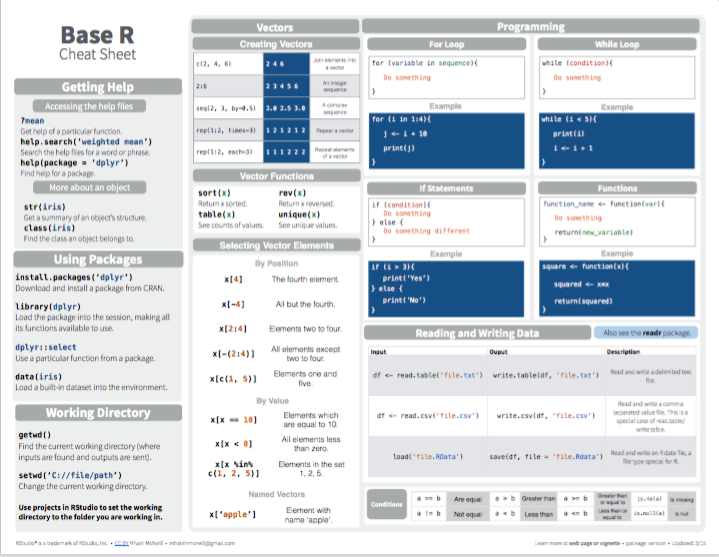
Figure 2.1: Base R summary from Posit cheatsheets.

• Advanced R:

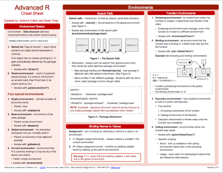
Figure 2.2: Advanced R summary from Posit cheatsheets.

Miscellaneous

Other helpful links that do not fit into the above categories include:

• R-bloggers collects blog posts on R.

• Quick-R (by Robert Kabacoff) is a popular website on R programming.

• R-exercises provides categorized sets of exercises to help people developing their R programming skills.

• A series of software reviews by Bob Muenchen at r4stats describes and evaluates alternative user environments for interacting with R.

2.5.3 Preview

In Chapter 3 on Data structures, we will encounter R data structures beyond linear vectors. More specifically, we will learn that atomic vectors can assume different shapes (e.g., as matrices) and can be combined into more complex data structures (e.g., lists and rectangular tables).

2.6 Exercises

The following exercises allow to verify your understanding on basic R concepts and commands:

Conceptual exercises

2.6.1 The ER of R

When discussing the fit between tools and tasks in Chapter 1, we encountered the notion of ecological rationality (ER, in Section 1.2.5). Now that we have learned some basic R concepts and commands, we can ask:

1. Where would R be located in Figure 1.7?

2. Where would we locate an individual R function?

3. How does the figure change when distinguishing between R (the language), RStudio (the IDE), or some R package?

Note: Try answering these questions in a few sentences, rather than optimizing your answers. Thinking too long about these issues can make us quite dizzy.

2.6.2 Data types and forms

Please answer the following questions in a few sentences:

1. Describe the similarities and differences between scalars and vectors in R.

2. What are the main data types in R? Which function(s) allow checking or verifying them for a given data object?

3. Describe the difference between logical and numeric indexing (of a vector) in your own words.

Practical exercises: Using R

The following exercises can be solved by using vectors as the only R data structure:

2.6.3 Recycling and indexing creatures

Assume we have the following data about a set of fictional creatures:

# Assume some data (a character vector of length 4): 
name   <- c("Axl", "Beatrice", "Sir Gawain", "Querig")
role   <- c("person", "person", "legendary knight", "dragon")
female <- c(FALSE, TRUE, FALSE, TRUE)
age    <- c(65, 60, 70, 800)

Tasks

Recycling

Predict, evaluate and explain the result of the following expressions:

• name == "Beatrice"
• name[female | age > 65]
• mean(age[role != "person"])

Indexing

Use a combination of vector indexing and R functions to answer the following questions:

• What is the name of the male person?
• What is the role of the creature whose name starts with the letter “Q”?
• What is the gender of the youngest creature?
• What is the mean age of all male creatures?

2.6.4 Familiar vectors

1. Create vectors that represent information about yourself and (at least four of) your family members:

• name (e.g., as given_name and family_name)
• relation to yourself (e.g., “mother”, “brother”, “grandfather”, etc.)
• gender (see Gender for options)
• date of birth (DOB, as a Date, like 2024-11-19, or as variables for year, month, day)
• height (in some unit)

Note: If you are concerned about your privacy, feel free to adopt the perspective of a member of some historic or public family (e.g., Charles III or Homer Simpson).

2. Describe your vectors in terms of their data types and shapes.

3. Use R functions (and vector indexing) to answer the following questions:

   • How many different family names are in the set?
   • Are there more males or more females in the set?
   • What is the mean height of the female family members?
   • Which family members are taller than yourself?
   • What is the age (in years) of each person?\(^{*}\)
   • Which proportion of them have already celebrated their birthday this year?\(^{*}\)
   • What is the mean age of the members with above-average height?

4. Try to find a way to represent the following information:\(^{*}\)

• Which foreign language(s) (lang) does each person speak?

What makes representing this information difficult? If it is not possible, why not (i.e., what prevents us from representing it)? If it is possible, how could we answer the following questions:

• How many foreign languages are spoken in the family?
• Who speaks French?
• Who speaks more than one foreign language?\(^{*}\)

Note: Solving these tasks requires looking up some R functions. The tasks marked with an asterisk (\(^{*}\)) are difficult to solve and require some auxiliary vectors and functions. If they are too difficult, try to state what you are missing (in terms of data types or shapes) for solving them.

2.6.5 Plotting fun

In Section 2.4.2, we explored the plot_fn() function of the ds4psy package to decipher its arguments. In this exercise, we explore the plot_fun() function of the same package.

1. Assume the perspective of an empirical scientist to explore the arguments of the plot_fun() function in a similar fashion.

library(ds4psy)  # loads the package

plot_fun()  # calls the function (with default arguments)

Hint: Solving this task essentially means to answer the question “What does this argument do?” for each argument (i.e., the lowercase letters from a to f, and c1 and c2).

2. Use your exploration of plot_fun() to reconstruct the command that creates the following plots:

Hint: Check the documentation of plot_fun() and colors() (e.g., for color information).

For additional exercises, see Chapter 1: Basic R concepts and commands of the ds4psy textbook (Neth, 2023a):

2.6.6 Cumulative savings

• See 1.8.4 Exercise 4

2.6.7 Vector arithmetic

• See 1.8.5 Exercise 5

2.6.8 Cryptic arithmetic

• See 1.8.6 Exercise 6

This concludes our exercises on basic R concepts and commands.

---

16. Assigning T and F to FALSE and TRUE, respectively, is a really bad idea, as T commonly denotes TRUE and F commonly denotes FALSE. However, the example shows that we must never rely on the single letters T and F being assigned to specific truth values.↩︎

17. Fun fact: The English writer Evelyn Waugh (1903–1966) and his wife Evelyn Gardner (1903–1994) had the same given name.↩︎

18. The main collection of available R packages (aka. libraries) is The Comprehensive R Archive Network (CRAN). Given an online connection, any package published there can be installed via the install.packages() command (or the Install button in the RStudio IDE). See Appendix B for resources on writing R packages.↩︎

19. In the old days, people used to get and read books to get this kind of information. One of the most astonishing things about R is that all of its documentation is already available on your computer when installing an R package.↩︎