24 R pour l’art
The process of preparing programs for a digital computer is especially attractive,
not only because it can be economically and scientifically rewarding, but also
because it can be an aesthetic experience much like composing poetry or music.Donald E. Knuth in his Preface to The Art of Computer Programming (1973)
We began Chapter 10 on Using colors by reflecting on the interactive and subjective nature of colors and art. If art is primarily viewed as an experience, it can encompass ways of expressing ourselves that do not result in artistic objects. A processual and interactive view of art is not new or revolutionary: We traditionally classify performances of dance, music or theater as works of art, although they do not produce artistic stuff that we can grasp and take home with us, or buy to exhibit on a pedestal or store away in a fire-proof safe.
A more controversial topic: Can computer code that mimics traditional artwork be considered art? If so, who is the artist — the programmer or the program? — and what constitutes the artistic process — the act of programming or the experience of its output? Recently, these questions have increased in urgency, as deep fakes and AI-generated artworks not only closely mimic and may surpass artwork created by humans, but raise deep questions regarding the nature of creativity and humanity.
Distinguish between two perspectives:
Computer programming as an activity that provides aesthetic experiences.
Using computer programming to create artistic expressions.
In the preface to The Art of Computer Programming (1973), Donald E. Knuth argued for 1. Just like scientists often take pleasure in discovering simplicity or symmetry in formal models, aiming for clarity, functionality, and efficiency when writing computer code appeals to many aspects of elegance and beauty. Simple proof of existence by someone reporting his or her experience.
The latter is clearly possible as well (e.g., when creating visualizations). As artists have always adopted and explored the limits of technology, it would be very surprising if an Albrecht Dürer or Leonardo da Vinci living today would advise us to abstain from using computers to create art. But the path from creative intent to an artistic end-result is complicated by many factors. For instance, judging artistic merit often depends less on the creator’s intentions than on the recipients viewing the resulting product.
Preflections
What could correspond to beauty in code?
What is art? Who evaluates its merits?
Map different data types to different types of (visual and non-visual) expression.
24.1 Introduction
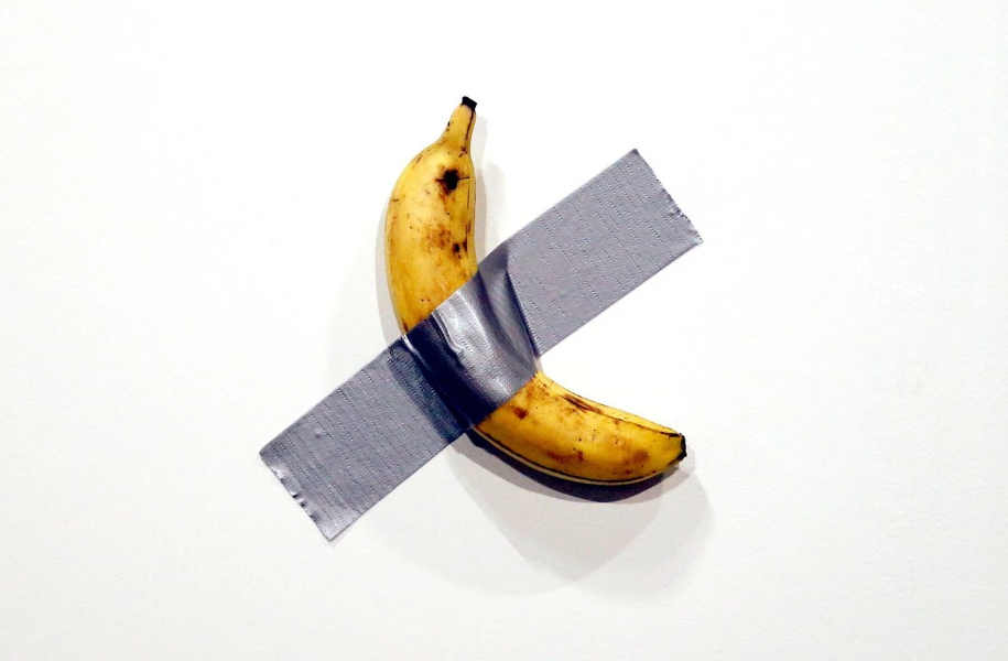
Figure 24.1: This piece of art sold for $120,000 before being eaten (NYT).
Art is hard — particularly when it looks simple. When seeing an ancient Greek statue or portrait by Rembrandt, it’s pretty easy to acknowledge that the artist was immensely capable. But especially when looking at modern art (see Figure 24.1), we often get the impression “I could do this myself”. However, when we are honest, we have to admit that our own imitations of Jackson Pollock’s paintings (see Wikipedia) never quite match the originals, and our shredded images or taped bananas get never sold at an auction. Thus, there are many things that sets art apart from non-art.
24.1.1 What is art?
What precisely counts as art is difficult or impossible to define. Rather than trying to define art, here’s a recent quote from Danielle Navarro’s blog post Art from code I (Navarro, 2024):
What about “art” – what counts as “art”? In this essay I will…
…just kidding. I do not have the arrogance to pretend that I know what art is.
Art is pretty (except when it isn’t). Art is created (except when it is found).
Art is intentional (except when it is accidental).
Art makes you think (sometimes, not always).
Art relies on artist skill (except when you send GPT-3 generated text to DALL-E).
Art is uniquely human (no it isn’t).
Art… yeah, look, I have no idea what art is. Personally, I like to make pretty things
from code that appeal to my aesthetic sensibilities, and that’s good enough for me.
As Danielle Navarro is not only a great data scientist, but also a truly inspiring artist (and a former professor of psychology), we take a break from our usual fable for definitions here. When creating pretty things is fun, who cares whether it qualifies as art?
Actually, one reason for the difficulty of defining art is the way in which art plays with (and often frustrates) our expectations. This illustrates that art — beyond being a huge cultural and social phenomenon — is also a matter of psychology: If someone put the Mona Lisa in a box (or wrapped a building in cloth), nobody would see it. Art depends on being experienced and interpreted, thus partly becomes constructed in the mind of its recipient.
To render the concept of computer art more plausible, we point out some relations between art and mathematical models.
24.1.2 Encoded art?
Geometry is an area of mathematics that describes the properties of objects in space.
Perhaps the most immediate association when mentioning computers in the context of art:
Mathematical descriptions of aesthetic properties (in terms of numbers and numerical relations) promise to “decode” art.
Example of the golden ratio (see Wikipedia), which is closely connected to the Fibonnaci sequence (see Wikipedia) and fractal geometry.
Hope of discovering the underlying mechanisms that govern many processes in nature and natural laws of beauty.
However, beyond numbers and the mathematics of art, there are many other links, once we allow ourselves to adopt different perspectives on the properties of data and code.
Different types of objects:
- Objects in computer code (data types and structures) vs.
- visual objects (printed text, images, sculptures) vs.
- non-visual objects (words, but also sounds and tunes).
Text as a complex mix of features:
- Text as data: characters, words, paragraphs, etc. vs.
- Text as a collection of visual objects, with specific colors, shapes, sizes, etc.
24.2 Visualizing structure
Examples of visualizing regularity and randomness: Revealing patterns and processes.
Organization of section: From regularity/order to irregularity/chaos.
Goal: Not developing artwork, but methods for creating visual objects.
However, we will realize that the dichotomy regularity vs. randomness quickly breaks down: Many seemingly chaotic processes obey laws that can be described and seen. Aesthetic experience of beauty involves a mix of regularity and randomness: order vs. chaos.
24.2.1 Circles and squares
Plotting simple geometric objects as a pre-requisite for more complex compositions.
Plot outlines and random points on these outlines.
Practice task: Plotting points (or other shapes) on a circle.
24.2.2 Mathematical patterns
Regularity can be quite charming.
Task: Arrange points within a circle.
An example inspired by nature: Arrangement of sunflower seeds.
Figure 24.2 provides an example image:
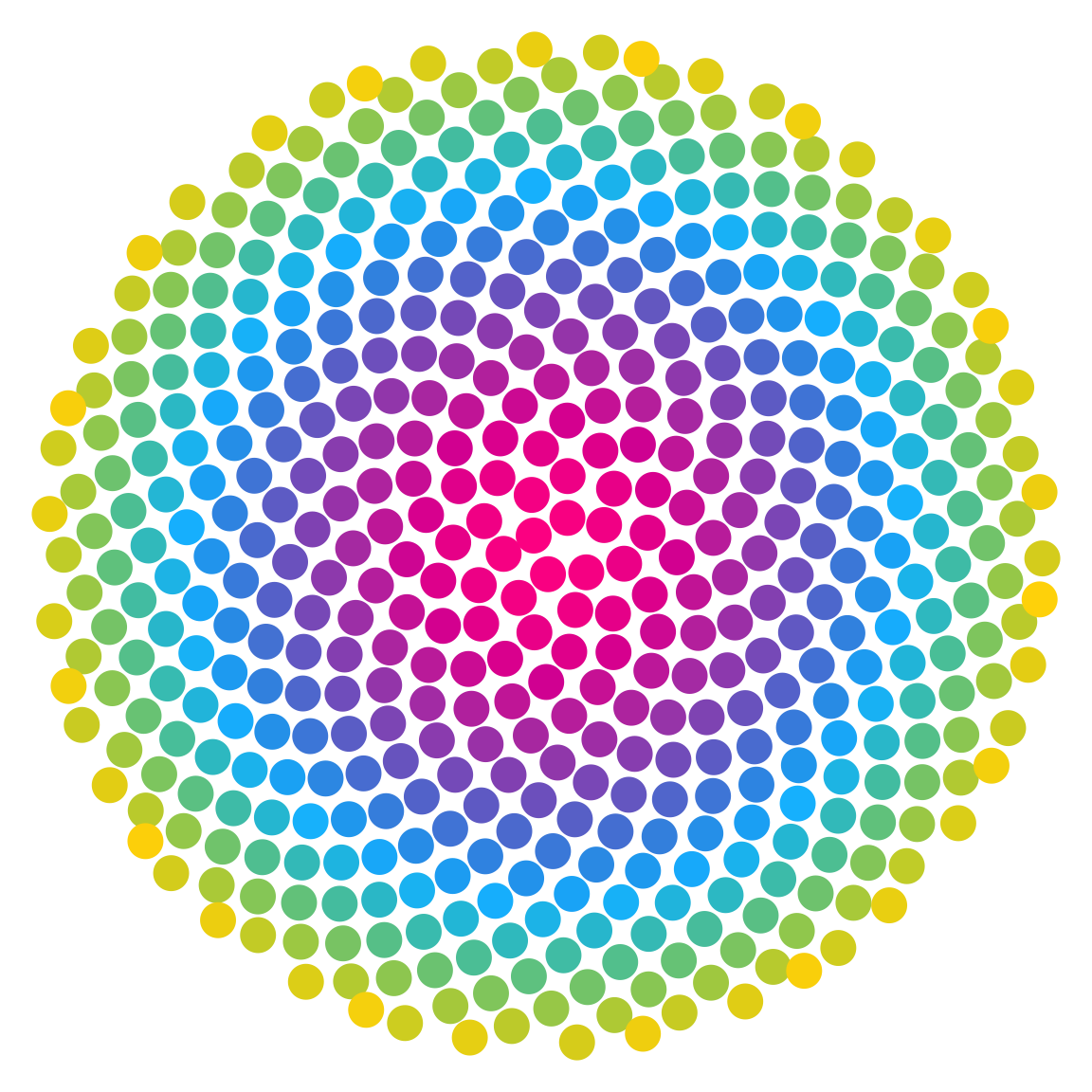
Figure 24.2: Plotting a pattern of points inspired by nature.
24.3 Plotting text
Text is usually used to convey messages and meanings (semantics). As a common data type, the representation of text (as symbols with a syntax) provides interesting challenges and opportunities to data analysts (see Chapter 17). This section aims to show that playing with the visual aspects of text can also yield aesthetic effects.
24.3.1 The task
Challenge: Plot text (as a visualization) and provide some statistics about character or word frequency.
Seems simple, but realize: Many plotted images are no longer text, but pixel-based (each location has a color value).
Use an example text.
As an example, we can use the bardr package (Billings, 2021) to load William Shakespeare’s complete works and extract the famous Sonnet 18 (see Wikipedia):
# Get some literary work:
library(bardr)  # the complete works of William Shakespeare, as provided by Project Gutenberg

# Extract some work: Poetry > Sonnet 18
works  <- all_works_df
poetry <- subset(works, works$genre == "Poetry")
sonnet_18_start <- grep("compare thee to a summer", poetry$content)            # find 1st line
sonnet_18 <- poetry$content[(sonnet_18_start - 1):(sonnet_18_start + 14 - 1)]  # extract sonnet
sonnet_18 <- gsub(pattern = "\\\032", replacement = "'", x = sonnet_18)        # corrections
text <- sonnet_18

## Write text to file:
# cat(sonnet_18, file = "bard.txt", sep = "\n")- Figure 24.3 shows the sonnet text, as plotted by the
plot_text()function of the ds4psy package (Neth, 2025b):
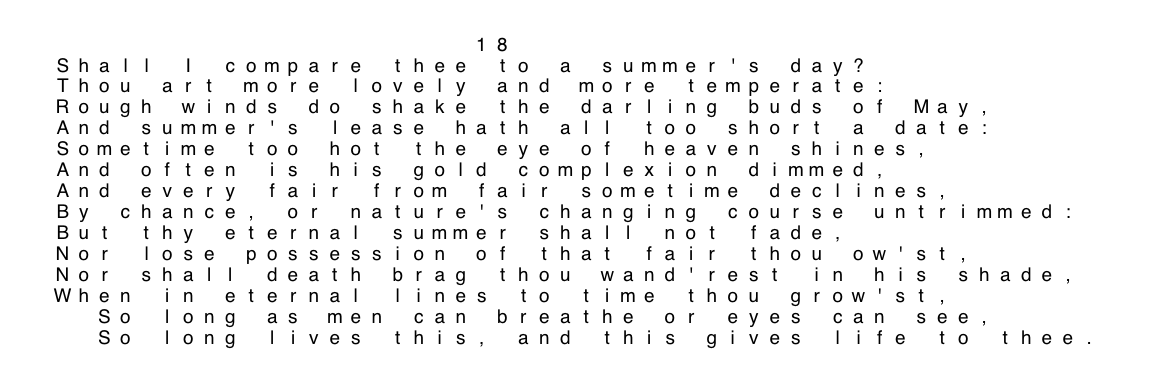
Figure 24.3: Visualizing Shakespeare’s Sonnet 18 (using the plot_charmap() function of ds4psy).
24.3.2 Plot text
Basic question: Text as strings of words, sentences, or paragraphs, or as a collection of individual characters?
Here: Individual characters (i.e., on a grid of x/y-locations, similar to crossword puzzles).
- Advantage: Easy to place words, as each character has a unique coordinate.
- Disadvantage: Equidistant spacing creates a grid-like appearance.
Data structure: Table of individual characters char, plus their x- and y-locations.
Goal:
#>   char x y
#> 1    S 1 1
#> 2    h 2 1
#> 3    a 3 1
#> 4    l 4 1
#> 5    l 5 1
#> 6      6 1
Subtasks
- Turn the text (provided as a character vector with one element per line of text) into a vector of individual characters.
#>  [1] "                    18"
#>  [2] "Shall I compare thee to a summer's day?"
#>  [3] "Thou art more lovely and more temperate:"
#>  [4] "Rough winds do shake the darling buds of May,"
#>  [5] "And summer's lease hath all too short a date:"
#>  [6] "Sometime too hot the eye of heaven shines,"
#>  [7] "And often is his gold complexion dimmed,"
#>  [8] "And every fair from fair sometime declines,"
#>  [9] "By chance, or nature's changing course untrimmed:"
#> [10] "But thy eternal summer shall not fade,"
#> [11] "Nor lose possession of that fair thou ow'st,"
#> [12] "Nor shall death brag thou wand'rest in his shade,"
#> [13] "When in eternal lines to time thou grow'st,"
#> [14] "  So long as men can breathe or eyes can see,"
#> [15] "  So long lives this, and this gives life to thee."
#> [1] "S" "h" "a" "l" "l" " "
#> [1] " " "t" "h" "e" "e" "."
Ad 1: Note that both are character vectors, but of different lengths.
- Generate the x- and y-coordinates for individual characters.
Ad 2: Mapping increasing coordinates to rows and positions in text.
We could use a combination of 2 loops that iterate through each line of text and each individual character per line. However, we can also use a single loop (for each line of text) and use numerical indexing to map the coordinates for the characters within the current line.
(See map_text_coord() definition.)
Result:
#>   char x y
#> 1    S 1 1
#> 2    h 2 1
#> 3    a 3 1
#> 4    l 4 1
#> 5    l 5 1
#> 6      6 1
24.3.3 Adding counts and colors
While such visualizations can be aesthetically pleasing, combining them with quantitative aspects (e.g., counting pattern matches) may also enable new insights.
Subtasks
- Count character frequency
Result:
#> chars
#>  e  o  t  s  a  h  n  r  i  l  m  d  u  f  g  c  y  '  v  p  S  w  A  b  B  N
#> 63 44 39 38 37 31 31 28 26 23 22 20 13 10 10  9  8  6  5  4  4  4  3  3  2  2
#>  1  8  I  k  M  R  T  W  x
#>  1  1  1  1  1  1  1  1  1
Map frequency value to each character in the char vector (i.e., a typical join() or merge()` problem).
- Map the frequency values to an appropriate color palette
# (a) Frequency map:
fm <- count_chars_words(x = text[-1])
names(fm) <- c("chars", names(fm)[-1])
dim(cm)
#> NULL
head(fm)
#>   chars char_freq  word word_freq
#> 1     S         4 Shall         1
#> 2     h        31 Shall         1
#> 3     a        37 Shall         1
#> 4     l        23 Shall         1
#> 5     l        23 Shall         1
#> 6             104              NA

# (b) Char map:
cm <- map_text_coord(x = text[-1], flip_y = TRUE)
cm$ix <- 1:nrow(cm)  # add row nr
dim(cm)
#> [1] 612   4
head(cm)
#>   char x  y ix
#> 1    S 1 14  1
#> 2    h 2 14  2
#> 3    a 3 14  3
#> 4    l 4 14  4
#> 5    l 5 14  5
#> 6      6 14  6

# (c) Combine:
tb <- cbind(cm, fm)
dim(tb)
#> [1] 612   8
head(tb)
#>   char x  y ix chars char_freq  word word_freq
#> 1    S 1 14  1     S         4 Shall         1
#> 2    h 2 14  2     h        31 Shall         1
#> 3    a 3 14  3     a        37 Shall         1
#> 4    l 4 14  4     l        23 Shall         1
#> 5    l 5 14  5     l        23 Shall         1
#> 6      6 14  6             104              NA

# Check:
all(tb$char == tb$chars)
#> [1] TRUE
Plot text with character/word statistics:
- Show character frequency (using a continuous color scale):
ggplot(tb, aes(x = x, y = y)) +
  # geom_tile(aes(fill = word_freq)) +
  geom_text(aes(label = char, col = char_freq), fontface = 1) +
  scale_color_gradient(low = "grey90", high = "black") +
  # coord_equal() +
  theme_classic()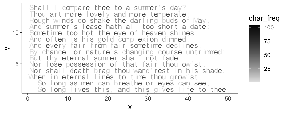
Figure 24.4: Text with character frequency.
Using factor(char_freq) for an ordinal color scale:
ggplot(tb, aes(x = x, y = y)) +
  # geom_tile(aes(fill = word_freq)) +
  geom_text(aes(label = char, col = factor(char_freq)), fontface = 1) +
  # scale_color_gradient(low = "grey90", high = "black") +
  scale_color_manual(values = usecol(c("grey90", "black"), n = length(unique(factor(tb$char_freq))))) +
theme_classic()- Figure 24.5 shows a version generated by varying the color and label rotation options of
plot_chars():
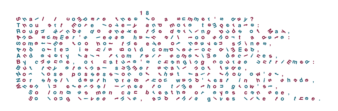
Figure 24.5: Varying label colors and angles in Shakespeare’s Sonnet 18 (using the plot_chars() function of ds4psy).
- If we want to locate and highlight specific target terms, we can use the regular expression options provided by the
plot_chars()function (see Figure 24.6):
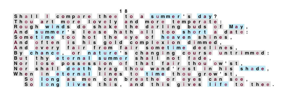
Figure 24.6: Locating and visualizing pattern matches in Shakespeare’s Sonnet 18 (using the plot_chars() function of ds4psy).
Note that all these plots are character-based: The basic unit is an individual character and all characters have the same width and height. In formatted text (e.g., when using real typesetting systems, e.g., TeX), not all characters have the same length. This would require a different approach to plotting text (see e.g., the text decoration functions in the unikn package). But even when plotting longer strings (i.e., entire words or sentences), the plotted text still changes its format by becoming part of an image. Thus, real desktop imaging software disinguishes text from graphical objects for as long as possible and only converts text into a graphical format when necessary (e.g., for printing it).
Nevertheless, our examples show that the boundaries between plain text and graphics are easily blurred, especially when we start thinking about word search problems, crossword puzzles, or word clouds. Thinking about new ways of visual expression will also change the ways we see characters and texts.
24.3.4 Extensions
-
Creating word search puzzles:
- start with a \(m \times\ n\) grid of
NAvalues and
- a list of words to place.
- specify orientation: 2 directions (fw/bw), 4 orientations (horizontal, vertical, 2 diagonals)
- aim to place elements (under constraints)
- fill rest so that no new words are created
- start with a \(m \times\ n\) grid of
24.4 Conclusion
If we see art as a process, an experience, an attitude or a perspective, anything can qualify. But rather than encouraging arbitrary or random variations, successful works of art must bridge various oppositions: The act of creation must result in a fitting output and the objective product must reliably evoke a matching subjective experience. Thus, much like in an act of successful communication, the ecological rationality of art consists in the correspondence between signal and receiver, medium and message. The intellectually stimulating controversy regarding the artistic merit of computer-generated art does not need to limit us. Fortunately, if we truly enjoy creating something, we do not need to worry about its eventual evaluation.
24.4.2 Resources

Some pointers to resources for inspirations and ideas:
Artists
Some personal favorites:
- Paul Klee:
- Grenzen des Verstandes, 1927, Bayerische Staatsgemäldesammlungen - Sammlung Moderne Kunst in der Pinakothek der Moderne München (updated 19.06.2023)
- Das Urweltpaar, 1921, Bayerische Staatsgemäldesammlungen - Sammlung Moderne Kunst in der Pinakothek der Moderne München (updated 19.06.2023)
- Tanz des trauernden Kindes II, 1922, Bayerische Staatsgemäldesammlungen - Sammlung Moderne Kunst in der Pinakothek der Moderne München (updated 19.06.2023)
Inspirations
The works of the following artists are sources of admiration and inspiration:
Antonio Sánchez Chinchón: https://fronkonstin.com and https://github.com/aschinchon
Marcus Volz: https://marcusvolz.com/ and https://github.com/marcusvolz
Lijia Yu: Making Visual Illusions in R: http://yulijia.net/vistat/2013/03/make-visual-illusions-in-r
Vít Gabrhel: Blog post on Getting started with generative art in R
Danielle Navarro: Data science blog, gallery of generative art and corresponding code repositories (e.g.,
bursts, flametree, stalk-and-feather, tangle, unboxing).Dan Gries: https://dangries.com blog RectangleWorld and its examples of generative art
Thomas Lin Pedersen: Generative art is a generative artist based in Denmark, but also the developer of many R packages (see his Data imaginist blog for details)
Readings
Articles and books with inspirations and related ideas:
See the foreword to the Strange attractors (1993) book by Julien C. Sprott at http://sprott.physics.wisc.edu/sa.htm.
Books by Clifford Pickover (on chaos, fractals, patterns, etc.), see http://www.pickover.com.
24.5 Exercises

Exercises on R pour l’art:
24.5.1 Visualizing mathematical puzzles
The so-called Collatz conjecture (see Wikipedia sounds like a simple math problem:
Starting with a positive integer \(n\), compute the following numbers by:
- If the current number \(n\) is even, compute the \(n+1\). number as \(3n + 1\);
- If the current number \(n\) is odd, compute the \(n+1\). number as \(n/2\).
and repeat these rules to compute the next numbers.
The Collatz conjecture claims that regardless of its initial value \(n\), the sequence will always reach 1.
Once a sequence reaches the value \(4\), the sequence would get stuck in an infinite loop:
\(4\) (even): \(4/2 = 2\) (even): \(2/2 = 1\) (odd): \(3+1 = 4\), etc.
Hence, the condition of reaching the value of 1 stops the procedure, and will be met when reaching a value of 2 or 4.
Your tasks:
Write an R function that returns the sequence for a given input value \(n\).
Create a visualization that illustrates the sequences or some of their properties for a range of starting values.
Assume you wanted to verify the conjecture for a large number of initial values \(n\) (e.g., \(n = 1, 2, ... 10^{10}\)). How could you make this more efficient than simply running your function for every candidate value?
Hint: The following video clip from the Veritasium channel explains the problem, provides some history, and contains lots of inspiring visualizations:
Solution
A corresponding function could use a while loop or use recursion.
- ad 1: A solution that uses a
whileloop (and considers some special cases):
Collatz <- function(n){

  # Initialize:
  seq <- n
  target <- +1

  # Catch some cases of special inputs:
  if (n == 0){
    stop("n = 0 would create an infinite loop.")
  } else if (!ds4psy::is_wholenumber(n)){
    stop("n is no integer, contrary to assumptions...")
  } else if (n < 0){
    warning("n < 0, contrary to assumptions. Checking for -1.")
    target <- -1
  }

  # Loop:
  while (n != target) {

    # Apply rules:
    if (n %% 2 == 0){  # x is even:
      n <- n/2
    } else if (n %% 2 == 1){ # x is odd:
      n <- 3 * n + 1
    }

    # Add n to seq:
    seq <- c(seq, n)

  } # while end.

  return(seq)

}

# Check:
Collatz(1)
#> [1] 1
Collatz(2)
#> [1] 2 1
Collatz(3)
#> [1]  3 10  5 16  8  4  2  1
Collatz(15)
#>  [1]  15  46  23  70  35 106  53 160  80  40  20  10   5  16   8   4   2   1
Collatz(27)
#>  [1]   27   82   41  124   62   31   94   47  142   71  214  107  322  161  484
#> [16]  242  121  364  182   91  274  137  412  206  103  310  155  466  233  700
#> [31]  350  175  526  263  790  395 1186  593 1780  890  445 1336  668  334  167
#> [46]  502  251  754  377 1132  566  283  850  425 1276  638  319  958  479 1438
#> [61]  719 2158 1079 3238 1619 4858 2429 7288 3644 1822  911 2734 1367 4102 2051
#>  [ reached getOption("max.print") -- omitted 37 entries ]

# Note that function works for negative integers:
Collatz(-4)
#> [1] -4 -2 -1
# but: Collatz(-5) gets stuck in a loop.
Collatz(-6)
#> [1] -6 -3 -8 -4 -2 -1

# Note errors for:
# Collatz(NA)
# Collatz(0)
# Collatz(1/2)

# Apply to range of values:
# sapply(X = 1:30, FUN = Collatz)- As all numbers in the sequence follow the same rules, we can also create a recursive function (without considering cases of non-standard inputs):
Collatz_rec <- function(n){

  if (n == 1) {

    seq <- n  # stopping case

  } else {

    # Apply rules:
    if (n %% 2 == 0){  # n is even:

      n_new <- n/2

    } else if (n %% 2 == 1){  # n is odd:

      n_new <- 3 * n + 1

    }

    # Recursive step:
    seq <- c(n, Collatz_rec(n_new))

  }

  return(seq)

}

# Check:
Collatz_rec(1)
#> [1] 1
Collatz_rec(9)
#>  [1]  9 28 14  7 22 11 34 17 52 26 13 40 20 10  5 16  8  4  2  1

# Apply to range of values:
# sapply(X = 1:30, FUN = Collatz_rec)- ad 3: There are many ways of writing more efficient functions. A key idea is that we do not need to (re-)check any number that occurs in a sequence that is known to conform to the conjecture. Thus, after checking a sequence and verifying that it reaches 1, we can add all its numbers to a store of “known numbers”. As soon as a sequence reaches any known number, we can stop checking it.
24.5.2 Visualizing word frequency
- Our example of plotting text in Section 24.3 used color to visualize the frequency of each character. Extend the example to visualize the frequency of words in a text.
Solution
Highlighting word frequency (using tb from above):
ggplot(tb, aes(x = x, y = y)) +
  geom_tile(aes(fill = word_freq)) +
  geom_text(aes(label = char), col = "white", fontface = 1) +
  scale_fill_continuous(low = "thistle3", high = "darkmagenta",
                        # low = "red3", high = "darkred",
                        # low = "deepskyblue", high = "darkslateblue",
                        guide = "colorbar", na.value = "white") +
  # coord_equal() +
  theme_classic()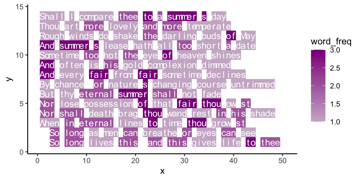
Figure 24.7: Text with word frequency highlightening.