3 R data structures

This chapter continues our basic introduction to R (R Core Team, 2024). More specifically, this chapter introduces data structures that reach beyond vectors (introduced in Chapter 2). As we will see, these other data structures either shape or combine vectors into more complex structures.

Important concepts and contents on this chapter include:

• defining different data structures (generalizing from vectors to matrices, arrays and tables, and from lists to data frames);
• accessing and changing data structures by (numeric or logical) indexing or subsetting, or by referring to element names.

Preparation

Recommended readings for this chapter include:

• Chapter 1: Basic R concepts and commands of the ds4psy book (Neth, 2023a)

Preflections

Before reading on, please take some time to reflect upon the following questions:

• In which forms can variables of different types be stored?

• Which differences exist between a (linear) vector and a (rectangular) matrix or table?

• Which properties of a vector are too limited for representing real-world data?

Note: This chapter is still fragmentary. See Chapter 1: Basic R concepts and commands of the ds4psy book (Neth, 2023a) for a more complete account.

3.1 Introduction

In Chapter 2, we learned that mastering R (or any other programming language) essentially consists in solving two inter-related tasks (see Section 2.1):

1. Representing various types of information as objects (Section 2.2.1).

2. Using functions for manipulating those objects (Section 2.4).

We further learned that every data object has a shape and type and encountered some of R’s key data types (or modes, see Section 2.2.2).

A key limitation of Chapter 2 was that we used linear vectors as the only shape of data object. While a vector can have any of the key data types, its shape is characterized by its length (and vectors with only one element are called scalars).

In this chapter, we will encounter additional data structures (i.e., combinations of data shapes and types). As we will see, these structures build upon the elementary concept of a vector, but extend it by either changing its shape or combining multiple data types. First, our humble vector structure can be tweaked into more complex shapes to create matrices, arrays, or tables. And when we want to store more than a single data type, we turn to lists as linear data structures that can store multiple types of data. As a special case that is both convenient and important, data frames are rectangular data structures that can store vectors of a single or multiple data types.

3.1.1 Contents

This chapter extends Chapter 2 by introducing additional R concepts and commands. Its key concept is the notion of a data structure as a specific combination of data types and shapes. Beyond atomic vectors, we will learn to create and access lists, matrices, and data frames, plus briefly introduce arrays and tables.

3.1.2 Data and tools

This chapter only uses base R functions and snippets of example data that we will generate along the way.

3.2 Overview

In Chapter 2, we learned that data objects are characterized by their shape and by their type. To create and use more flexible and more powerful data objects, the construct of a “data structure” is helpful: Data structures are constructs that store particular combinations of data shapes and data types. The range of possible shapes of a data object is determined by its data structure, but data structures are more general constructs that affect both the shapes and types of data objects.

In R, different data structures are distinguished based on the fact whether they contain only a single or multiple data types. Thus, the columns of Table 3.1 distinguish between data structures for “homogeneous” vs. “heterogeneous” data types.

Table 3.1: Overview of R data structures (i.e., combinations of data shapes and data types).

Dimensions	Homogeneous data types	Heterogeneous data types
1D	atomic vector	list
2D	matrix	tabular (data frame/tibble)
nD	array/table

Although Table 3.1 contains five different data structures, two of them are by far the most important ones for our purposes:

• vectors are linear (1-dimensional) data structures. So-called atomic vectors only contain a single data type and have a length of 1 or more elements.

• tabular data structures are rectangular (2-dimensional) structures that can contain multiple data types (in different columns). The terms data frames and tibbles denote two slightly different types of tabular data structures.¹⁸

A good question is: Where are scalar objects in Table 3.1? The answer is: R is a vector-based language. Thus, even scalar objects are represented as (atomic, i.e., homogeneous) vectors (of length \(1\)).

3.3 Linear data structures

Atomic vectors and lists are both linear data structures insofar as they only have one dimension (1D) and are characterized by their length. However, atomic vectors and lists differ in the type(s) of data that they can accommodate:

• in atomic vectors, all elements are of the same data type

• in lists, elements can contain different data types

3.3.1 Atomic vectors

In Chapter 2, we discussed vectors as the primary data structure in R (see Section 2.3). To repeat, a vector is an ordered sequence of elements with three common properties:

1. its type of elements (tested by typeof());
   
2. its length (tested by length());
3. optional attributes or meta-data (tested by attributes()).

As a straightforward way of representing some facts about five people, we could store their name, gender, and age as vectors:

name   <- c("Adam", "Ben", "Cecily", "David", "Evelyn")
gender <- c("male", "male", "female", "male", "other")
age    <- c(21, 19, 20, 48, 45)

Here, name and gender are character vectors, whereas age is a numeric vector. The following expression creates a logical vector that indicates which values of age are at least 21 and the corresponding names:

age >= 21
#> [1]  TRUE FALSE FALSE  TRUE  TRUE
name[age >= 21] 
#> [1] "Adam"   "David"  "Evelyn"

If any of these terms are unclear, consider revisiting the introductory Chapter 2 on Vectors (Section 2.3) and logical indexing (Section 2.3.2).

The vast majority of vectors we encounter are atomic vectors (i.e., all elements of the same type), but lists are often used in R for storing a variety of data types in a common object (e.g., in statistical analyses). It is important to understand that the term “atomic” in “atomic vectors” refers to the type of the vector, rather than its shape or length: Atomic vectors can contain one or more objects of any type (i.e., can have multiple lengths), but not multiple types.

In the context of data structures, we extend the basic data structure of atomic vectors in several ways:

1. Lists are complex/hierarchical vectors that accept multiple data types

2. Matrices are atomic vectors with additional shape attributes

3. Rectangular tables (data frame and tibbles) are lists of atomic vectors

3.3.2 Lists

Beyond atomic vectors, R provides lists as yet another data structure to store linear sequences of elements. Internally, lists in R actually are vectors (see Wickham, 2014a for details).
However, rather than atomic vectors, lists are complex vectors (aka. hierarchical or recursive vectors) that can contain elements of multiple data types/modes and various shapes. Thus, the key feature of lists is that their elements can contain objects of different data types.

Defining lists

Lists are sequential data structures in which each element can have an internal structure. Thus, lists are similar to atomic vectors (e.g., in having a linear shape that is characterized by its length()). Crucially, different elements of a list can be of different data types (or modes). As every element of a list can also be a complex (rather than an elementary) object, lists are also described as “hierarchical” data structures.

We can create a list by applying the list() function to a sequence of elements:

# lists can contain a mix of data shapes:
l_1 <- list(1, 2, 3)     # 3 elements (all numeric scalars)
l_1
#> [[1]]
#> [1] 1
#> 
#> [[2]]
#> [1] 2
#> 
#> [[3]]
#> [1] 3

l_2 <- list(1, c(2, 3))  # 2 elements (of different lengths)
l_2
#> [[1]]
#> [1] 1
#> 
#> [[2]]
#> [1] 2 3

The objects l_1 and l_2 are both lists and contain the same three numeric elements, but differ in the representation’s shape:

• l_1 is a list with three elements, each of which is a scalar (i.e., vector of length 1).
  
• l_2 is a list with two elements. The first is a scalar, but the second is a (numeric) vector (of length 2).

Technically, a list is implemented in R as a vector of the mode “list”:

vl <- vector(length = 2, mode = "list")

is.vector(vl)
#> [1] TRUE
is.list(vl)
#> [1] TRUE

The fact that lists are also implemented as vectors (albeit hierarchical or recursive vectors) justifies the statement that vectors are the fundamental data structure in R.

Due to their hiearchical nature, lists are more flexible, but also more complex than the other data shapes we encountered so far. Unlike atomic vectors (i.e., vectors that only contain one type of data), lists can contain a mix of data shapes and data types. A simple example that combines multiple data types (here: “numeric”/“double” and “character”) is the following:

# lists can contain a multiple data types:
(l_3 <- list(1, "B", 3))
#> [[1]]
#> [1] 1
#> 
#> [[2]]
#> [1] "B"
#> 
#> [[3]]
#> [1] 3

The ability to store a mix of data shapes and types in a list allows creating complex representations. The following list contains both a mix of data types and shapes:

# lists can contain a mix of data types and shapes:
(l_4 <- list(1, "B", c(3, 4), c(TRUE, TRUE, FALSE)))
#> [[1]]
#> [1] 1
#> 
#> [[2]]
#> [1] "B"
#> 
#> [[3]]
#> [1] 3 4
#> 
#> [[4]]
#> [1]  TRUE  TRUE FALSE

As lists can contain other lists, they can be used to construct arbitrarily complex data structures (like tables or tree-like hierarchies):

# lists can contain other lists: 
l_5 <- list(l_1, l_2, l_3, l_4)

Finally, the elements of lists can be named. As with vectors, the names() function is used to both retrieve and assign names:

# names of list elements:
names(l_5)  # check names => no names yet: 
#> NULL

names(l_5) <- c("uno", "two", "trois", "four")  # assign names:

names(l_5)  # check names:
#> [1] "uno"   "two"   "trois" "four"

As with atomic vectors, two basic questions for working with lists are:

• How can we inspect a list?
• How can we access the elements of a list?

We will briefly introduce some functions for addressing these tasks.

Inspecting lists

The is.list() function allows checking whether some R object is a list:

is.list(l_3)  # a list
#> [1] TRUE
is.list(1:3)  # a vector
#> [1] FALSE
is.list("A")  # a scalar
#> [1] FALSE

Whereas atomic vectors are not lists, lists are also vectors (as lists are hierarchical vectors):

is.vector(l_3)
#> [1] TRUE

As lists are linear data structures, we can always inspect their length:

length(l_3)
#> [1] 3
length(l_4)
#> [1] 4

As the hierarchical nature of lists makes them objects with a potentially interesting structure, a useful function for inspecting lists is str():

str(l_3)
#> List of 3
#>  $ : num 1
#>  $ : chr "B"
#>  $ : num 3
str(l_4)
#> List of 4
#>  $ : num 1
#>  $ : chr "B"
#>  $ : num [1:2] 3 4
#>  $ : logi [1:3] TRUE TRUE FALSE

Lists are powerful structures for representing data of various types and shapes, but can easily get complicated. In practice, we will rarely need lists, as vectors and tables usually suffice for our purposes. However, as data frames actually are lists and we occasionally will encounter lists that are not data frames (e.g., as the output of statistical functions), it is good to be aware of lists and know how to access their elements.

Accessing list elements

As lists are implemented as vectors, accessing list elements is similar to indexing vectors, but needs to account for an additional layer of complexity. This is achieved by distinguishing between single square brackets (i.e., []) and double square brackets ([[]]):

• x[i] returns the i-th sub-list of a list x (as a list);

• x[[i]] removes a level of the hierarchy and returns the i-th element of a list x (as an object).

The distinction between single and double square brackets is important when working with lists:

• [] always returns a smaller (sub-)list, whereas
  
• [[]] removes a hierarchy level to return list elements.

Thus, what is achieved by [] with vectors is achieved by [[]] with lists. An example illustrates the difference:

l_4       # a list
#> [[1]]
#> [1] 1
#> 
#> [[2]]
#> [1] "B"
#> 
#> [[3]]
#> [1] 3 4
#> 
#> [[4]]
#> [1]  TRUE  TRUE FALSE
l_4[3]    # get 3rd sub-list (a list with 1 element)
#> [[1]]
#> [1] 3 4
l_4[[3]]  # get 3rd list element (a vector)
#> [1] 3 4

For named lists, there is another way of accessing list elements that is similar to accessing the named variables (columns) of a data frame:

• x$n selects a list element (like [[]]) with the name n.

# l_5      # a list with named elements
l_5$two    # get element with the name "two"
#> [[1]]
#> [1] 1
#> 
#> [[2]]
#> [1] 2 3

Importantly, using [[]] and $n both return list elements that can be of various data types and shapes. In the case of l_5, the 2nd element named “two” happens to be a list:

identical(l_5$two, l_5[[2]])
#> [1] TRUE

For additional details on lists, as well as helpful analogies and visualizations, see 20.5 Recursive vectors (lists) of r4ds (Wickham & Grolemund, 2017).

Using lists or vectors?

Due to their flexibility, any data structure used above can be re-represented as a list. For instance, the name or age vectors could easily be transformed into lists with 5 elements:

as.list(name)
as.list(age)

However, this re-representation would only add complexity without a clear benefit. As long as we just want to store elements of a single data type, using an atomic vector is not only sufficient, but simpler than and thus superior to using a list.

What could justify using a list? Like vectors, lists store linear sequences of elements. But lists are only needed when storing heterogeneous data, i.e., data of different types (e.g., numbers and text) or sequences of elements of different shapes (e.g., both scalars and vectors). For instance, statistical functions often use lists to return a lot of information about an analysis in one complex object.

From linear data structures (like atomic vectors and lists), it is only a small step to study rectangular data structures known as matrices and tables.

3.4 Rectangular data structures

Rectangular data structures generally store data in a two-dimensional (2D) format (i.e., a grid containing rows and columns). When all rows and all columns have the same length, the resulting structure has a rectangular shape.

As Table 3.1 has shown, we distinguish between two main types of 2D-data structures in R:

1. matrices are rectangular structures that are homogeneous with respect to their data (i.e., are atomic vectors with additional shape parameters).

2. tabular data structures also have a rectangular shape, but allow for heterogeneous data types (in different columns). The two main types of tabular data structures are data frames and tibbles.

The confusion regarding different 2D-data structures is clarified by distinguishing between their form and content: Matrices and rectangular tables both have a rectangular shape (i.e., rows and columns). However, matrices and rectangular tables differ with respect to their contents: Whereas a matrix is really an atomic vector (i.e., a data object allowing only for a single type) with additional shape attributes, a data frame or tibble is a more complex data structure that combines multiple vectors (i.e., allowing for different data types).

Beware of “tables”

We use the clumsy term “rectangular data structure”, as the shorter term “table” is vague and confusing. Whenever speaking of tables, we need to distinguish between the term’s meanings in general language and its specific instantiations as a data structure in R.

A confusing aspect is that the term table is sometimes used informally as a super-category for “any rectangular data structure” (i.e, data in the shape of a rectangle — or arranged in rows and columns — including data frames, matrices, or tibbles). Apart from the difference between matrices and data frames (which actually is a distinction between vectors and lists), R also distinguishes between rectangular data structures of type data.frame and others of type tibble. We ignore this distinction here, but note that tibbles are simpler data frames (see Chapter 12 for details).

As tables can extend in more than two dimensions, another term for multi-dimensional tables is an array. In R, however, objects of type “array” are essentially vectors (i.e., atomic) with additional shape attributes (i.e., the array’s dimensions). In R, the flexibility and vagueness of the term table is aggravated further, as R uses the data type table to denote a particular type of array (i.e., a multi-dimensional data structure that expresses frequency counts in a contingency table).

Overall, we see that the term table is used in many different ways and for different kinds of objects. When the object of reference is clear (e.g., when we are referring to a particular matrix, data frame, or tibble), calling it a “table” usually just refers to its rectangular shape (i.e., a data structure containing rows and columns). However, it generally makes sense to distinguish between matrices and data frames, which is why we will discuss these two types of tabular structures next.

3.4.1 Matrices

When a rectangular data structure contains a single type of data in all its cells (i.e., in all its rows and columns), we have a matrix of data. In R, a matrix really is an atomic vector that is tweaked into another shape (i.e., a re-shaped vector). Internally, this is implemented by taking a vector and adding attributes that describe its shape and the names of its rows or columns.

Creating matrices

A way of turning an atomic vector into a matrix is provided by the matrix() function. It takes one main argument for its data (i.e., the atomic vector) and several arguments that describe the shape of the desired matrix structure: Its number of rows nrow, its number of columns ncol, and a logical argument byrow that arranges data in a by-row or by-column fashion:

# Reshaping an atomic vector into a rectangular matrix:
(m1 <- matrix(data = 1:20, nrow = 5, ncol = 4, byrow = TRUE))
#>      [,1] [,2] [,3] [,4]
#> [1,]    1    2    3    4
#> [2,]    5    6    7    8
#> [3,]    9   10   11   12
#> [4,]   13   14   15   16
#> [5,]   17   18   19   20

(m2 <- matrix(data = 1:20, nrow = 5, ncol = 4, byrow = FALSE))
#>      [,1] [,2] [,3] [,4]
#> [1,]    1    6   11   16
#> [2,]    2    7   12   17
#> [3,]    3    8   13   18
#> [4,]    4    9   14   19
#> [5,]    5   10   15   20

Why would we want to re-shape vectores into a matrix? As we will see below, the main reason is that the rectangular shape allows new ways of accessing (sets of) data elements (by indexing rows, columns, or cells).

While it is important to remember that a matrix is really just an atomic vector with a different shape, we can create a matrix by combining multiple atomic vectors — provided that they have the same data type and (usually) the same length. Actually, we could first combine such vectors with the c() function and then re-shape the resulting vector with the matrix() function, but the following two vector binding-functions make this process more convenient:

• the rbind() function treats each vector as a row;

• the cbind() function treats each vector as a column:

# Create 3 vectors (of the same length and type): 
x <- 1:3
y <- 4:6
z <- 7:9

# Combining vectors (of the same length): ---- 
(m3 <- rbind(x, y, z))  # combine as rows
#>   [,1] [,2] [,3]
#> x    1    2    3
#> y    4    5    6
#> z    7    8    9

(m4 <- cbind(x, y, z))  # combine as columns
#>      x y z
#> [1,] 1 4 7
#> [2,] 2 5 8
#> [3,] 3 6 9

When the data to be shaped into a matrix does not match to each other or the size arguments, R tries to recycle vectors or truncates to the dimensions provided. Note that the following commands all create Warning messages, as the number of arguments do not fit together as a matrix (of the required size):

# Create 2 vectors (of the same type, but different lengths):
m <- 1:2
n <- 3:5

rbind(m, n)  # recycling m
#>   [,1] [,2] [,3]
#> m    1    2    1
#> n    3    4    5
cbind(m, n)  # recycling m
#>      m n
#> [1,] 1 3
#> [2,] 2 4
#> [3,] 1 5

matrix(data = 1:10, nrow = 3, ncol = 4)  # recycling data
#>      [,1] [,2] [,3] [,4]
#> [1,]    1    4    7   10
#> [2,]    2    5    8    1
#> [3,]    3    6    9    2
matrix(data = 1:10, nrow = 3, ncol = 3)  # truncating data
#>      [,1] [,2] [,3]
#> [1,]    1    4    7
#> [2,]    2    5    8
#> [3,]    3    6    9

The matrices m1 to m4 all contained numeric data. However, data of type “logical” or “character” can also stored in matrix form:

# A matrix of logical values:
(m5 <- matrix(data = 1:18 %% 4 == 0, nrow = 3, ncol = 6, byrow = TRUE))
#>       [,1]  [,2]  [,3]  [,4]  [,5]  [,6]
#> [1,] FALSE FALSE FALSE  TRUE FALSE FALSE
#> [2,] FALSE  TRUE FALSE FALSE FALSE  TRUE
#> [3,] FALSE FALSE FALSE  TRUE FALSE FALSE

# A matrix of character values:
(m6 <- matrix(sample(letters, size = 16), nrow = 4, ncol = 4, byrow = FALSE))
#>      [,1] [,2] [,3] [,4]
#> [1,] "u"  "d"  "s"  "a" 
#> [2,] "j"  "c"  "z"  "f" 
#> [3,] "m"  "b"  "e"  "w" 
#> [4,] "n"  "t"  "h"  "y"

Indexing matrices

In R, retrieving values from a matrix m — or other rectangular data structures — works similarly to indexing vectors. First, we will consider numeric indexing. Due to the two-dimensional nature of a matrix, we now need to specify two indices in square brackets: the number of the desired row, and the number of the desired column, separated by a comma. Thus, to get or change the value of row r and column c of a matrix m we can refer to m[r, c]. Just as with vectors, providing multiple numeric indices selects the corresponding rows or columns. When the value of r or c is left unspecified, all rows or columns are selected.

# Selecting cells, rows, or columns of matrices: ---- 
m1[2, 3]  # in m1: select row 2, column 3
#> [1] 7
m2[3, 1]  # in m2: select row 3, column 1
#> [1] 3

m1[2,  ]  # in m1: select row 2, all columns
#> [1] 5 6 7 8
m2[ , 1]  # in m1: select column 1, all rows
#> [1] 1 2 3 4 5

m3
#>   [,1] [,2] [,3]
#> x    1    2    3
#> y    4    5    6
#> z    7    8    9
m3[2, 2:3]  # in m3: select row 2, columns 2 to 3
#> [1] 5 6
m3[1:3, 2]  # in m3: select rows 1 to 3, column 2
#> x y z 
#> 2 5 8

m4[]  # in r4: select all rows and all columns (i.e., all of m4)
#>      x y z
#> [1,] 1 4 7
#> [2,] 2 5 8
#> [3,] 3 6 9

When retrieving specific elements of a vector, we could describe the desired elements by a logical expression (i.e., logical indexing). For instance, given the vectors name, gender and age from above, we can easily get the names of the male individuals or of those under the age of 21 by

name[gender == "male"]
#> [1] "Adam"  "Ben"   "David"
name[age < 21]
#> [1] "Ben"    "Cecily"

As matrices are vectors with a 2D-shape, logical indexing extends to matrices:

m4 > 5   # returns a matrix of logical values
#>          x     y    z
#> [1,] FALSE FALSE TRUE
#> [2,] FALSE FALSE TRUE
#> [3,] FALSE  TRUE TRUE
typeof(m4 > 5)
#> [1] "logical"
m4[m4 > 5]  # indexing of matrices (yields a vector):
#> [1] 6 7 8 9

Just as with vectors, we can apply functions to matrices. Typical examples include:

# Applying functions to matrices: ---- 
is.matrix(m1)
#> [1] TRUE
typeof(m2)
#> [1] "integer"

# Note the difference between: 
is.numeric(m3) # type of m3? (1 value)
#> [1] TRUE
is.na(m3)      # NA values in m3? (many values)
#>    [,1]  [,2]  [,3]
#> x FALSE FALSE FALSE
#> y FALSE FALSE FALSE
#> z FALSE FALSE FALSE

# Computations with matrices: 
sum(m1)
#> [1] 210
max(m2)
#> [1] 20
mean(m3)
#> [1] 5
colSums(m3)  # column sums of r3
#> [1] 12 15 18
rowSums(m4)  # row sums of r4
#> [1] 12 15 18

Just as length() provides crucial information about a vector, some functions are specifically designed to provide the dimensions of rectangular data structures:

ncol(m4)  # number of columns 
#> [1] 3
nrow(m4)  # number of rows
#> [1] 3
dim(m4)   # dimensions as vector c(rows, columns)
#> [1] 3 3

A typical function in the context of matrices is t() for transposing (i.e., swap the rows and columns of) a matrix:

t(m4)
#>   [,1] [,2] [,3]
#> x    1    2    3
#> y    4    5    6
#> z    7    8    9
t(m5)
#>       [,1]  [,2]  [,3]
#> [1,] FALSE FALSE FALSE
#> [2,] FALSE  TRUE FALSE
#> [3,] FALSE FALSE FALSE
#> [4,]  TRUE FALSE  TRUE
#> [5,] FALSE FALSE FALSE
#> [6,] FALSE  TRUE FALSE

3.4.2 Practice

The following practice exercises allow you to check your understanding of this section.

Creating matrices

1. Above, we created two matrices m3 and m4 by binding three vectors into the rows or columns of a matrix:

# Create 3 vectors (of the same length and type): 
x <- 1:3
y <- 4:6
z <- 7:9

# Combining vectors (of the same length): ---- 
(m3 <- rbind(x, y, z))  # combine as rows
#>   [,1] [,2] [,3]
#> x    1    2    3
#> y    4    5    6
#> z    7    8    9
(m4 <- cbind(x, y, z))  # combine as columns
#>      x y z
#> [1,] 1 4 7
#> [2,] 2 5 8
#> [3,] 3 6 9

• Create two identical matrices m3b and m4b without using the rbind() and cbind() functions.

Hint: The text above mentioned that we can replace the binding commands by using the c() and matrix() functions.

Solution

It is easy to combine the c() and matrix() functions to create two matrices with the same data cells as m3 and m4:

# Combine c() and matrix() to re-create matrices:
(m3b <- matrix(data = c(x, y, z), nrow = 3, byrow = TRUE))
#>      [,1] [,2] [,3]
#> [1,]    1    2    3
#> [2,]    4    5    6
#> [3,]    7    8    9
(m4b <- matrix(data = c(x, y, z), ncol = 3, byrow = FALSE))
#>      [,1] [,2] [,3]
#> [1,]    1    4    7
#> [2,]    2    5    8
#> [3,]    3    6    9

However, note that the matrices m3 and m4 additionally contain the variables of its component vectors as the row or column names of the matrix. Manually replicating this automatic behavior of rbind() and cbind() is more difficult, as it requires dealing with the list elements of dimnames():

row.names(m3b)     <- c("x", "y", "z")
dimnames(m4b)[[1]] <- c("x", "y", "z")
all.equal(m3, m3b)
#> [1] TRUE

dimnames(m4b)[[2]] <- c("x", "y", "z")
all.equal(m4, m4b)
#> [1] "Attributes: < Component \"dimnames\": Component 1: target is NULL, current is character >"

2. Predict and explain what happens if we tried to combine the following three vectors into a matrix:

# Create 3 vectors (of the same length): 
X <- 1:3
Y <- letters[4:6]
Z <- 7:9 %% 2 == 0

# Combining vectors (of the same length): ---- 
rbind(X, Y)
cbind(X, Z)
cbind(X, Y, Z)

Solution

The key insight here is that the three atomic vectors share the same length, but contain different types. However, an R matrix can only contain a single data type. Which common type this is depends on the data types that are being combined. Combining any data type with characters yields characters, but logical values can turn into numbers or characters.

Accessing and evaluating matrices

Assuming the definitions of the matrices m5 and m6 from above, i.e.,

m5
#>       [,1]  [,2]  [,3]  [,4]  [,5]  [,6]
#> [1,] FALSE FALSE FALSE  TRUE FALSE FALSE
#> [2,] FALSE  TRUE FALSE FALSE FALSE  TRUE
#> [3,] FALSE FALSE FALSE  TRUE FALSE FALSE
m6
#>      [,1] [,2] [,3] [,4]
#> [1,] "u"  "d"  "s"  "a" 
#> [2,] "j"  "c"  "z"  "f" 
#> [3,] "m"  "b"  "e"  "w" 
#> [4,] "n"  "t"  "h"  "y"

• Predict, evaluate, and explain the result of the following R expressions:

m5[2, 6]
m5[2, ]
m5 == FALSE
sum(m5)
t(t(m5))

m6[2, 3]
m6[ , 4]
m6[nrow(m6), (ncol(m6) - 1)]
m6 == "e"
toupper(m6[4, ])

3.4.3 Data frames

Table 2.1 (in Section 2.3.2) was rectangular in containing three rows (with values for the variables name, gender, and age) and five columns (one for each person, plus an initial column indicating the variable name of in each row). This is a perfectly valid table, but not the type of tabular data structure typically used in R. Tabular data structures in R typically combine several vectors into a larger data structure, but use the individual vectors as columns, rather than as rows. Such a by-column combination of vectors is shown in Table 3.2:

Table 3.2: The same facts about five people (as a table with 5 rows and 3 columns).

name	gender	age
Adam	male	21
Ben	male	19
Cecily	female	20
David	male	48
Evelyn	misc	45

Importantly, Table 3.2 provides exactly the same information as Table 2.1 — and as its three constituent vectors name, gender, and age — but in a tabular shape that uses the vectors as its columns, rather than as its rows.

As (atomic) vectors in R need to have the same data type (e.g., name contains character data, whereas age contains numeric data), the information on each person — due to containing multiple data types — cannot be stored as a vector. Instead, we represent each person as a row (aka. an observation) of the table.

Creating data frames

To create a data frame, we first need the data to be framed in some other form. The most typical scenario is that we have the data as a set of vectors. If these vectors have the same length, creating a data frame from vectors can be achieved by the data.frame() function. For instance, we can define a data frame df from our name, gender, and age vectors (from Section 2.3.2) by assigning it to data.frame(name, gender, age):

# 3 variables (as vectors):
name   <- c("Adam", "Ben", "Cecily", "David", "Evelyn")
gender <- c("male", "male", "female", "male", "other")
age    <- c(21, 19, 20, 48, 45)

(df <- data.frame(name, gender, age))
#>     name gender age
#> 1   Adam   male  21
#> 2    Ben   male  19
#> 3 Cecily female  20
#> 4  David   male  48
#> 5 Evelyn  other  45

A remarkable fact about data frame df is that it is an object that combines and contains multiple data types. Internally, R represents a data frame as a list of atomic vectors. The vectors form the columns of the data frame df, rather than its rows. Note that we could have assigned our new data frame to an object named some_data or five_people, but the name df is often used as a short and convenient name for a data frame that can be poked and probed later.

The data.frame() function is quite powerful and coerces a variety of objects into data frames. For instance, we can use it to turn individual vectors or matrices into data frames:

# Creating data frames from a vector or matrix: 
v <- 1:9
m <- matrix(v, nrow = 3)

data.frame(v)  # from a vector
#>   v
#> 1 1
#> 2 2
#> 3 3
#> 4 4
#> 5 5
#> 6 6
#> 7 7
#> 8 8
#> 9 9
data.frame(m)  # from a matrix
#>   X1 X2 X3
#> 1  1  4  7
#> 2  2  5  8
#> 3  3  6  9

Due to the rectangular shape of a data frame, its columns all need to have the same length. If the vectors used to create a data frame do not have the same length, the shorter one(s) are recycled to the length of the longest one:

# From vectors of different length: 
abc <- letters[1:3]
data.frame(v, abc)
#>   v abc
#> 1 1   a
#> 2 2   b
#> 3 3   c
#> 4 4   a
#> 5 5   b
#> 6 6   c
#> 7 7   a
#> 8 8   b
#> 9 9   c

If the vector lengths are not compatible (in the sense: can the shortest vector be recycled to the length of the longest vector?), combining vectors by df() would yield an error.

Applying functions to data frames

As data frames are ordinary objects in R, we do things with them by applying functions to them. As Chapter 2 emphasized that every R object is characterized by its type and shape, we can ask:

• What is the type of the data frame df?
• What is the shape of the data frame df?

The data type question was answered above: As data frames are objects that combine multiple data types, R represents them as a list of atomic vectors. We can apply standard functions to obtain this information from our data frame df:

# df type:
is.data.frame(df)
#> [1] TRUE
typeof(df)
#> [1] "list"

For linear data structures (like vectors or lists), basic shape information is provided by their length(). For rectangular data structures (like matrices or data frames), we can still ask about their length(), but the more informative function provides their dimensions dim(). The two dimensions of a data frame can directly be queried by the nrow() and ncol() functions:

# df shape:
length(df)  # number of vectors/columns  
#> [1] 3
dim(df)     # dimensions 
#> [1] 5 3

nrow(df)   # == dim[1]
#> [1] 5
ncol(df)   # == dim[2] == length(df)
#> [1] 3

R provides many additional functions that work with data frames or their components (i.e., the data stored in them). However, when applying functions to data frames, we always need to consider what type of data is stored in them. Whereas some functions are generic (i.e., work with any type of data), others require specific data types. For instance, applying the is.na() function to a data frame works similar to applying it to a vector. But instead of providing a logical value for each vector element, it provides a logical value for each cell in the rectangular data frame. By contrast, arithmetic functions — like sum(), or more specialized versions like rowSums() and colSums() — will only work with numeric data types. The following illustrates this for a data frame dx that is created from a matrix mx:

# Create a matrix:
mx <- matrix(1:9, nrow = 3, byrow = TRUE)
mx[2, 2] <- NA  # change 1 element to a "missing value"

# As data frame:
dx <- data.frame(mx)
dx  # Note row and column names
#>   X1 X2 X3
#> 1  1  2  3
#> 2  4 NA  6
#> 3  7  8  9

# Applying generic function to dx:
dim(dx)
#> [1] 3 3
is.na(dx)
#>         X1    X2    X3
#> [1,] FALSE FALSE FALSE
#> [2,] FALSE  TRUE FALSE
#> [3,] FALSE FALSE FALSE

# Functions for numeric data types:
sum(dx, na.rm = TRUE)
#> [1] 40
rowSums(dx, na.rm = TRUE)
#> [1]  6 10 24
colSums(dx, na.rm = TRUE)
#> X1 X2 X3 
#> 12 10 18

As data frames are the most common way of storing data in R, there is a special form of indexing that allows accessing the variables of a data frame (i.e., the columns of a data frame) as vectors.

Name-based indexing of data frames

When a table tb has column names (e.g., a column called name), we can retrieve the corresponding vector by name-based indexing (aka. name indexing). This is the most convenient and most frequent way of accessing variables (i.e., columns) of tabular data structures (e.g., data frames). To use this form of indexing, we use a special dollar sign notation: Adding $ and the name of the desired variable name to the table’s object name tb yields its column name as a vector. This sounds complicated, but is actually very easy:

tb$name

In case of our data frame df, we can access its 1st and 2nd columns by their respective names:

names(df)  # prints the (column) names
#> [1] "name"   "gender" "age"

df$name
#> [1] "Adam"   "Ben"    "Cecily" "David"  "Evelyn"
df$gender
#> [1] "male"   "male"   "female" "male"   "misc"

Note that the last two expressions (with the $ notation) yield the corresponding columns of df as vectors. (Internally, the data frame is stored as a list of vectors and $ allows accessing list elements by their name.)

Numeric and logical indexing data frames

As data frames are lists of vectors, everything we have learned about numeric and logical indexing of vectors and matrices (above) also applies to data frames. Thus, we can also use numerical indexing on a data frame, just as with matrices (above). For instance, to get all rows of the first column, we can specify the data frame’s name, followed by [ , 1]:

df[ , 1]  # get (all rows and) the 1st column of df
#> [1] "Adam"   "Ben"    "Cecily" "David"  "Evelyn"
df[ , 2]  # get (all rows and) the 2nd column of df 
#> [1] "male"   "male"   "female" "male"   "misc"

Thus, these two expressions retrieve the 1st and 2nd column of the data frame df_1 (as vectors), respectively. As this is a very common task in R, there is an easier way of accessing the variables (columns) of a data frame.

Logical indexing on data frames is particularly powerful in allowing us to select particular rows (based on conditions specified on columns of the same data frame):

df[df$gender == "male", ]
#>    name gender age
#> 1  Adam   male  21
#> 2   Ben   male  19
#> 4 David   male  48
df[df$age < 21, ]
#>     name gender age
#> 2    Ben   male  19
#> 3 Cecily female  20

Note that the different types of indexing can be flexibly combined. For instance, the following command uses

• logical indexing (to select rows of df with an age value below 30)
• numerical indexing (to select only columns 1 and 2)
• name indexing (to get the variable name, as a vector), and
• numerical indexing (to select the 3rd element of this vector):

df[df$age < 30, c(1, 2)]$name[3]
#> [1] "Cecily"

In practice, such complex combinations are rarely necessary or useful. For instance, the following expressions retrieve the exact same result as the complex one, but have much simpler semantics:

df[3, 1]
#> [1] "Cecily"
df$name[3]
#> [1] "Cecily"

As data frames are lists, we can access their elements as we access list elements:

Adding variables (as columns)

To create an object in R, we learned that we simply need to name and assign some data to it. When applied to data frames, this usually implies that we want to add new variables as new columns. For instance, if we knew the height of each person in df, we could add this information as a new numeric vector:

height_in_ft <- c(6.2, 5.8, 5.2, 6.0, 5.7)
df$height_ft <- height_in_ft 

Similarly, if we had and wanted to add information which of the people in df had a valid driver’s license, we could define this information as a logical vector (with the same number of elements as people) and assign this vector to a new named variable of df:

# New df variable (as logical):
df$may_drive <- c(TRUE, FALSE, TRUE, FALSE, TRUE)

Assigning new colums to df changes the shape of the data frame:

dim(df)
#> [1] 5 5
ncol(df)
#> [1] 5

so that it now contains 5 columns:

Table 3.3: More facts about five people (as a table with 5 rows and 5 columns).

name	gender	age	height_ft	may_drive
Adam	male	21	6.2	TRUE
Ben	male	19	5.8	FALSE
Cecily	female	20	5.2	TRUE
David	male	48	6.0	FALSE
Evelyn	other	45	5.7	TRUE

A common way of adding new variables to a data frame consists in evaluating existing variables and adding the result of this evaluation as new variables. For instance, if we wanted to determine which people in df were allowed to drink alcohol in most U.S. states (i.e., are at least 21 years old) we could compute and directly add this information as follows:

# New df variable (based on existing variable):
df$may_drink <- df$age >= 21

As the result of the expression df$age >= 21 is a vector of logical values, the new variable df$may_drink is of type logical. But variables of other data types can be added in the same way. For instance, if we wanted to convert each person’s height from feet and inches into some metric unit (e.g., centimeters), we could extract the necessary information from the vector df$height_ft and add the result of our computation as a new column df$height_cm:

# Auxiliary vectors:
height_feet             <- df$height_ft %/% 1      # integers denote feet 
height_remaining_inches <- df$height_ft %% 1 * 10  # decimals denote inches
height_in_inches        <- (12 * height_feet) + height_remaining_inches  # 12 inches = 1 foot

# New df variable (based on auxiliary vector):
df$height_cm <- height_in_inches * 2.54  # 1 inch = 2.54 cm

As the three auxiliary vectors were based on df$height_ft, we could have performed the entire computation in a single step:

# New df variable (based on df$height_ft):
df$height_cm <- ((12 * df$height_ft %/% 1) + (df$height_ft %% 1 * 10)) * 2.54  # 1 inch = 2.54 cm

but using the auxiliary vectors made the steps more transparent. After computing and adding the new variables, our data frame df has grown futher to now contain 7 columns:

Table 3.4: Even more facts about five people (as a table with 5 rows and 7 columns).

name	gender	age	height_ft	may_drive	may_drink	height_cm
Adam	male	21	6.2	TRUE	TRUE	187.96
Ben	male	19	5.8	FALSE	FALSE	172.72
Cecily	female	20	5.2	TRUE	FALSE	157.48
David	male	48	6.0	FALSE	TRUE	182.88
Evelyn	other	45	5.7	TRUE	TRUE	170.18

As we now can access cells, rows, and columns of data frames (by name, numerical or logical indexing) and change existing or add new variables (by assigning values to existing or new variables), we are now in a position to perform powerful computations with data frames. To achieve this, we the rest of this book will increase our repertoire of functions that operate on data frames and their components.

When working with data, we will also encounter a variant of a data frame that is called a tibble. Tibbles are essentially a simpler type of data frame that is preferred in tidyverse contexts (Wickham et al., 2019) and created by the tibble package (Müller & Wickham, 2023). At this point, we only need to know that both data frames and tibbles are rectangular data structures that can store multiple data types as a list of vectors (see Chapter 12 for details).

Using lists or data frames?

Knowing that data frames are lists may suggest that it does not matter whether we use a data frame or a list to store data. This impression is false. Although it is possible to store many datasets as both as a list or a rectangular table, it is typically better to opt for the simpler format that is supported by more tools.

In principle, data frames and lists can store the same data (and even are variants of the same R data structure, i.e., a list). However, pragmatic reasons tip the balance in favor of data frames in most use cases: Whenever a set of vectors to be combined all have the same length, their combination would create a rectangular shape. As many R functions assume or are optimized for rectangular data structures, using data frames is typically the better choice.

The lesson to be learned here is that we should aim for the simplest data structure that matches the properties of our data. Although lists are more flexible than data frames, they are rarely needed in applied contexts. As a general rule, simpler structures are to be preferred to more complex ones:

• For linear sequences of homogeneous data, vectors are preferable to lists.

• For rectangular shapes of heterogeneous data, data frames are preferable to lists.

Thus, as long as data fits into the simple and regular shapes of vectors and data frames, there is no need for using lists. Vectors and data frames are typically easier to create and use than corresponding lists. Additionally, many R functions are written and optimized for vectors and data frames, rather than lists. As a consequence, lists should only be used when data requires mixing both different types and shapes of data, or when data objects get so complex, irregular, or unpredictable that they do not fit into a rectangular table.

Strings as factors

Note that the data.frame() function has an argument stringsAsFactors. This argument determines whether so-called string variables (i.e., of data type “character”) are converted into factors (i.e., categorical variables, which are internally represented as integer values with text labels) when generating a data frame. To the chagrin of generations of R users, the default of this argument used to be TRUE for several decades — which essentially meant that any character variable in a data frame was converted into a factor unless the user had specified stringsAsFactors = FALSE. As this caused much confusion, the default has been changed with the release of R version 4.0.0 (on 2020-04-24) to stringsAsFactors = FALSE. This shows that the R gods at https://cran.r-project.org/ are responding to user feedback. However, as any such changes are unlikely to happen quickly, it is safer to explicitly set the arguments of a function. To see the difference between both settings, consider the following example:

df_1 <- data.frame(name, gender, age, 
                   stringsAsFactors = FALSE)  # new default (since R 4.0.0+)
df_2 <- data.frame(name, gender, age, 
                   stringsAsFactors = TRUE)   # old default (up to R 3.6.3)

# Both data frames look identical:
df_1  
#>     name gender age
#> 1   Adam   male  21
#> 2    Ben   male  19
#> 3 Cecily female  20
#> 4  David   male  48
#> 5 Evelyn   misc  45
df_2
#>     name gender age
#> 1   Adam   male  21
#> 2    Ben   male  19
#> 3 Cecily female  20
#> 4  David   male  48
#> 5 Evelyn   misc  45

Printing the two data frames df_1 and df_2 shows us no difference between them. However, as the first two variables (i.e., name and gender) were string variables (i.e., of type “character”), they are represented as factors in df_1 versus remained character variables in df_2.

Let’s retrieve the first column of each data frame (as a vector). Using named indexing, we can easily retrieve and print the first column (i.e., with a name of name) of either data frame:

df_1$name
#> [1] "Adam"   "Ben"    "Cecily" "David"  "Evelyn"
df_2$name
#> [1] Adam   Ben    Cecily David  Evelyn
#> Levels: Adam Ben Cecily David Evelyn

Note the differences in the printed outputs. The output of df_1$name looks just any other character vector (with five elements, each consisting of a name). By contrast, the output of df_2$name also prints the same names, but without the characteristic double quotes around each name, and with a second line starting with “Levels:” before seeming to repeat the names of the first line. Before clarifying what this means, check the other variable in both df_1 and df_2 that used to be a character vector gender:

df_1$gender
#> [1] "male"   "male"   "female" "male"   "misc"
df_2$gender
#> [1] male   male   female male   misc  
#> Levels: female male misc

Again, df_1$gender appears to be a characer vector, but df_2$gender has been converted into something else. This time, the line beginning with “Levels:” only contains each of the gender labels once, and in alphabetical order.

In case you’re not confused yet, compare the outputs of the following commands:

typeof(df_1$name)
#> [1] "character"
typeof(df_2$name)
#> [1] "integer"

Whereas df_1$name was to be expected to be of type character, it should come as a surprise to see that df_2$name is of type integer. Given that df_2$name contains integers, we might be tempted to try out arithmetic functions like:

max(df_2$name)
sum(df_2$name)
mean(df_2$name)

If we try to evaluate these expressions, we get either Warnings or Error messages. How can we make sense of all this?

The magic word here is factor. As the stringsAsFactors = TRUE suggests, the character strings of the name and gender vectors have been converted into factors when defining df_2. Factors are categorical variables that only care about whether two values belong to the same or to different groups. Actually, R iternally encodes them as numeric values (integers) for each factor level. But as we never want to calculate with these numeric values (as they have no meaning beyond being either the same or different), they are also assigned a label, which is shown when printing the values of a factor.

A quick way of checking that we are dealing with a factor is the is.factor() function:

is.factor(df_1$name)
#> [1] FALSE
is.factor(df_2$name)
#> [1] TRUE

is.factor(df_1$gender)
#> [1] FALSE
is.factor(df_2$gender)
#> [1] TRUE

Factor variables are often useful (e.g., for distinguishing between groups in statistical designs). But it is premature to assume that any character variable should be a factor when including the variable in a data frame. Thus, it is a good thing that the default argument in the data.frame() function has been changed tostringsAsFactors = FALSE` in R v4.0.0.
Whoever needs factors can still get and use them — but novice users no longer need to deal with them all the time.

3.4.4 Practice

Creating data frames

1. Above, we combined three vectors into a matrix as follows:

# Create 3 vectors (of the same length): 
X <- 1:3
Y <- letters[4:6]
Z <- 7:9 %% 2 == 0

# Combining vectors (of the same length): ---- 
cbind(X, Y, Z)

• Why would we normally not want this matrix? What is the key advantage of data.frame(X, Y, Z)?

2. An alternative way to combine the same three vectors into a matrix is as follows:

# Combining vectors (of the same length): ---- 
rbind(X, Y, Z)

• This matrix has the same main problem (but different attributes and contents) as the matrix created by cbind(X, y, Z). But why can we no longer fix its problem by turning it into a data frame?

Computing with data frames

Using the data frame dx (from above),

dx
#>   X1 X2 X3
#> 1  1  2  3
#> 2  4 NA  6
#> 3  7  8  9

• predict, evaluate, and explain the result of the following expressions:

1. dim(dx)[1] == length(dx)
2. sum(!is.na(dx))
3. range(dx)
4. mean(dx$X3)
5. range(dx[3, ])

Solutions

dim(dx)[1] == length(dx)
#> [1] TRUE
sum(!is.na(dx))
#> [1] 8
range(dx)
#> [1] NA NA
mean(dx$X3)
#> [1] 6
range(dx[3, ])
#> [1] 7 9

Numeric indexing of data frames

Assuming the data frame df_2 (from above),

df_2
#>     name gender age
#> 1   Adam   male  21
#> 2    Ben   male  19
#> 3 Cecily female  20
#> 4  David   male  48
#> 5 Evelyn   misc  45

• predict, evaluate and explain the result of the following expressions (in terms of numeric indexing):

1. df_2[]

2. df_2[ , 1]

3. df_2[1:nrow(df_2), c(1)]

4. df_2[nrow(df_2):1, c(1)]

5. df_2[rep(1, 3), c(1, 2)]

6. df_2$name[3]

7. What do the following expressions do?

df_2[1:nrow(df_2), 1:ncol(df_2)]
df_2[1:nrow(df_2), ncol(df_2):1]
df_2[nrow(df_2):1, ncol(df_2):1]

Solutions

df_2[]
#>     name gender age
#> 1   Adam   male  21
#> 2    Ben   male  19
#> 3 Cecily female  20
#> 4  David   male  48
#> 5 Evelyn   misc  45
df_2[ , 1]
#> [1] Adam   Ben    Cecily David  Evelyn
#> Levels: Adam Ben Cecily David Evelyn
df_2[1:nrow(df_2), c(1)]
#> [1] Adam   Ben    Cecily David  Evelyn
#> Levels: Adam Ben Cecily David Evelyn
df_2[nrow(df_2):1, c(1)]
#> [1] Evelyn David  Cecily Ben    Adam  
#> Levels: Adam Ben Cecily David Evelyn
df_2[rep(1, 3), c(1, 2)]
#>     name gender
#> 1   Adam   male
#> 1.1 Adam   male
#> 1.2 Adam   male
df_2$name[3]
#> [1] Cecily
#> Levels: Adam Ben Cecily David Evelyn

ad 7.: The 3 expressions all return different variants of df_2 (or “representational isomorphs” of the same data). The 3 variants are being created by numeric indexing and differ in the order in which the rows of df_2, its columns, or both, are being sorted.

Logical indexing of data frames

Assuming the data frame df_1 (from above):

df_1
#>     name gender age
#> 1   Adam   male  21
#> 2    Ben   male  19
#> 3 Cecily female  20
#> 4  David   male  48
#> 5 Evelyn   misc  45

1. Predict, evaluate and explain what happens when evaluating the following expressions (in terms of logical indexing):

df_1[ , 3] > 30
df_1[df_1$age > 30, ]
df_1[df_1$gender != "male", c(1, 3, 2)]
df_1$name[df_1$gender == "male"]
sum(df_1$age[df_1$gender == "male"])

Data frames with factors

Given that our definition of df_2 (from above) used stringsAsFactors = TRUE:

1. Predict, evaluate and explain what happens in the following expressions:

nchar(as.character(df_2$name[3]))
as.numeric(df_2$name[3]) + 1
mean(as.numeric(df_2$name))

2. Why would the following expressions (which are simpler variants of the last three expressions) yield errors or warnings?

nchar(df_2$name[3])
df_2$name[3] + 1
mean(df_2$name)

3. What would happen, if the same expressions were used on df_1 (from above)?

nchar(df_1$name[3])
df_1$name[3] + 1
mean(df_1$name)

Computing and adding new variables

For the data frame df (above), add new variables to answer the following questions:

• Which people are identified as non-male?
• Which people are younger than average?
• Which people may drive but not drink?
• What is the average height of the people who may drink but not drive?
• Compute each person’s height_in_inches from df$height_cm.
• Re-compute df$height_ft_2 from height_in_inches and verify that it matches df$height_ft.

3.5 Multidimensional data structures

When introducing matrices (in Section 3.4.1 above), we noted that a matrix is simply a vector with a different shape. A matrix arranges the elements of a vector in two dimensions (i.e., rows and columns), but there is no reason to limit these shapes to two dimensions (i.e., 2D). Data structures that arrange data in more than two dimensions in R are the array and the table.

3.5.1 Array

An array in R simply is a multi-dimensional vector — a vector with a non-linear shape. From being a vector, it follows that arrays can only contain one type of data. We can create an array from a vector by the array() function:

# Create a vector:
(abc <- letters[1:12])
#>  [1] "a" "b" "c" "d" "e" "f" "g" "h" "i" "j" "k" "l"

# Create an array: 
(a_1 <- array(data = abc))
#>  [1] "a" "b" "c" "d" "e" "f" "g" "h" "i" "j" "k" "l"

Although the two objects abc and a_1 are both of type character and contain the same elements (i.e., the letters a to l), they differ in some respect: abc is a vector, but a_1 is an array:

is.vector(abc)
#> [1] TRUE
is.vector(a_1)
#> [1] FALSE

is.array(abc)
#> [1] FALSE
is.array(a_1)
#> [1] TRUE

Somewhat confusingly, both abc and a_1 have the same length. However, a_1 contains an additional dim attribute that describes its shape:

length(abc)
#> [1] 12
length(a_1)
#> [1] 12

dim(abc)
#> NULL
dim(a_1)
#> [1] 12

attributes(abc)
#> NULL
attributes(a_1)
#> $dim
#> [1] 12

By default, the dimensions dim of an array are set to length(data) (i.e., for a_1, the length of our abc vector). By setting dim to other values, we can create more complex arrays. As the dim argument is provided as a vector that specifies the number of elements per dimension, the number of array dimensions is determined by length(dim). For instance, a matrix is merely a special kind of (2D-)array:

# Create a 2d array:
(a_2 <- array(data = abc, dim = c(3, 4)))
#>      [,1] [,2] [,3] [,4]
#> [1,] "a"  "d"  "g"  "j" 
#> [2,] "b"  "e"  "h"  "k" 
#> [3,] "c"  "f"  "i"  "l"

is.matrix(a_2)
#> [1] TRUE
is.array(a_2)
#> [1] TRUE

Providing more than two dimensions creates multi-dimensional arrays that are no longer matrices:

# Create a 3d array:
(a_3 <- array(data = abc, dim = c(2, 3, 2)))
#> , , 1
#> 
#>      [,1] [,2] [,3]
#> [1,] "a"  "c"  "e" 
#> [2,] "b"  "d"  "f" 
#> 
#> , , 2
#> 
#>      [,1] [,2] [,3]
#> [1,] "g"  "i"  "k" 
#> [2,] "h"  "j"  "l"

is.matrix(a_3)
#> [1] FALSE
is.array(a_3)
#> [1] TRUE

Overall, an array in R is similar to a vector, but with a non-linear shape that is specified by an additional dim attribute.

Creating arrays by evaluating array() with data and dim arguments raises the question: What happens, when the (product of) dim does not correspond to the (length of) data? Let’s try:

(a_4 <- array(data = abc, dim = c(2, 2)))
#>      [,1] [,2]
#> [1,] "a"  "c" 
#> [2,] "b"  "d"
(a_5 <- array(data = abc, dim = c(3, 3, 2)))
#> , , 1
#> 
#>      [,1] [,2] [,3]
#> [1,] "a"  "d"  "g" 
#> [2,] "b"  "e"  "h" 
#> [3,] "c"  "f"  "i" 
#> 
#> , , 2
#> 
#>      [,1] [,2] [,3]
#> [1,] "j"  "a"  "d" 
#> [2,] "k"  "b"  "e" 
#> [3,] "l"  "c"  "f"

We see that the elements of abc are either truncated (if they do not fit into the shape defined by dim, as in a_4) or recycled (if length(data) is lower than the number of positions in the shape defined by dim, as in a_5).

Working with arrays essentially involves the same operations as any other R data types — accessing their elements and applying functions to them. Numeric indexing extends the logic of rectangular tables (with 2 indices) to additional dimensions by specifying as many indices as there are array dimensions:

# Numeric indexing of arrays:
a_3[1, 3, 2]  # 1 element: row 1, col 3, layer 2
#> [1] "k"
a_3[1,  ,  ]  # 1st row, all columns, all layers
#>      [,1] [,2]
#> [1,] "a"  "g" 
#> [2,] "c"  "i" 
#> [3,] "e"  "k"
a_3[ , 2,  ]  # 2nd column, all rows, all layers 
#>      [,1] [,2]
#> [1,] "c"  "i" 
#> [2,] "d"  "j"
a_3[ ,  , 2]  # 2nd layer, all rows, all columns 
#>      [,1] [,2] [,3]
#> [1,] "g"  "i"  "k" 
#> [2,] "h"  "j"  "l"

Note that failing to provide a specific number for a dimension (but providing the comma) yields all elements of the corresponding dimension and the objects returned from indexing arrays can be vectors, matrices, or arrays.

Some useful standard functions when working with an array are:

# Useful functions:
typeof(a_3)
#> [1] "character"
length(a_3)
#> [1] 12
dim(a_3)
#> [1] 2 3 2

"c" %in% a_3
#> [1] TRUE
"x" %in% a_3
#> [1] FALSE

Although dim can contain an arbitrary number of dimensions, humans typically find it difficult to keep track of more than three dimensions. Hence, most programmers may occasionally use 3D-arrays, but arrays with 4 or more dimensions are much rarer.

Another feature of arrays in R is that their dimensions can have names (set by the dimnames argument, as a list, so that both the dimension and their levels can be named). The main advantage of naming dimensions is that this additionally allows accessing array contents by their verbal labels. But as arrays are multi-dimensional vectors, most programmers refrain from naming their dimensions and use numerical indexing to access their contents. This differs for a special type of R array that is — somewhat confusingly — called a table.

3.5.2 Table

The R data structure table must not be confused with a rectangular table shape (i.e., data arranged in rows and columns, see above). Instead, an R table is a special type of array — a (potentially) multi-dimensional data structure that contains the counts of all category combinations of its dimensions.

As an example, imagine that we represented data about a group of people on three variables:

• gender: (e.g., male, female, or other)
• age: (e.g., in years, minor or adult, or as old vs. young)
• height (e.g., in some unit, or as short vs. tall)

Note the difference between categorical and continuous variables: Whereas some variables are categorical (like gender or may_drive), continuous variables (like age or height) can be turned into categorical variables.¹⁹ For instance, we could re-code and extract some categorical variables from our data frame df (from above):

df
#>     name gender age height_ft may_drive may_drink height_cm
#> 1   Adam   male  21       6.2      TRUE      TRUE    187.96
#> 2    Ben   male  19       5.8     FALSE     FALSE    172.72
#> 3 Cecily female  20       5.2      TRUE     FALSE    157.48
#> 4  David   male  48       6.0     FALSE      TRUE    182.88
#> 5 Evelyn  other  45       5.7      TRUE      TRUE    170.18

# Turn "age" into a binary category:
df$age_category[df$age >= mean(df$age)] <- "old"
df$age_category[df$age <  mean(df$age)] <- "young"

# Turn "height" into a binary category:
df$height_category[df$height_cm >= mean(df$height_cm)] <- "tall"
df$height_category[df$height_cm <  mean(df$height_cm)] <- "short"

# Select some variables (columns):
(df_3 <- df[, c(2, 8, 9)])
#>   gender age_category height_category
#> 1   male        young            tall
#> 2   male        young           short
#> 3 female        young           short
#> 4   male          old            tall
#> 5  other          old           short

Note that the partial data frame df_3 is more abstract than df by only containing categorical information on each individual, rather than person-identifying information (e.g., their name or some other identifier). When arranging the three variables as the orthogonal axes in three dimensions, we get a three-dimensional table. In R, such cross-tabulations of variable levels over two or more dimensions can be created by the table() function and represented as a table:

table(df_3)
#> , , may_drive = FALSE
#> 
#>         age_category
#> gender   old young
#>   female   0     0
#>   male     1     1
#>   other    0     0
#> 
#> , , may_drive = TRUE
#> 
#>         age_category
#> gender   old young
#>   female   0     1
#>   male     0     1
#>   other    1     0

Each cell in this table describes the frequency of a unique combination of variable values in our data (e.g., 1 older male individual that is tall). As each cell contains the frequency count of a combination of variable levels (or factors), such data structures are called contingency tables. The information contained in an R table can always be re-represented as a data frame with a frequency variable:

data.frame(table(df_3))
#>    gender age_category height_category Freq
#> 1  female        older           short    0
#> 2    male        older           short    0
#> 3   other        older           short    1
#> 4  female      younger           short    1
#> 5    male      younger           short    1
#> 6   other      younger           short    0
#> 7  female        older            tall    0
#> 8    male        older            tall    1
#> 9   other        older            tall    0
#> 10 female      younger            tall    0
#> 11   male      younger            tall    1
#> 12  other      younger            tall    0

Thus, an R table is a numeric array that provides compact and convenient representations of contingency information (i.e., information on the frequency of category combinations). When many category combinations are rare, the corresponding table becomes sparsely populated or patchy. This is further aggravated when including continuous variables. In the extreme, including a variable that uniquely identifies each case (like a name, address, or numeric identifier) implies that the frequency value of the corresponding category combination is 1, and most other category combinations will remain empty. Thus, the multi-dimensional table structure mostly makes sense for adopting an abstract perspective on contingency information — and even then we can always represent the same information in rectangular form.

Overall, uses of the R data structures array and table are relatively rare and limited to special cases. This may be partly due with the fact that multi-dimensional data structures are difficult to represent in human minds, although R provides powerful functions for computing or collapsing across their margins. Additionally, even when multi-dimensional representations make sense, we usually have ways of formatting the same information as rectangular tables or as lists (e.g., by adding variables or by introducing conventions, like triplets of color values, see Chapter 10). Thus, using vectors and data frames will suffice for the vast majority of use cases, and only some technical tasks (e.g., mathematical computations and complex simulations) may require additional data structures.

3.5.3 Practice

Although we will not be working much with arrays and tables in this course, here are some basic practice exercises for those data structures.

Working with arrays

1. How many elements are contained in an \(m \times n \times o\) array?

2. Assuming a_3 (from above), what are the elements, types, and shapes of

   • a_3[3]
     
   • a_3[1, 2, 1]
   • a_3[1, , ]

3. Assuming abc (from above), what are the elements, types, and shapes of

   • array(abc, dim = c(12, 1, 1))
   • array(abc, dim = c( 1, 12, 1))
   • array(abc, dim = c( 1, 1, 3))
   • array(abc, dim = c( 3, 3, 3))

Working with tables

A notorious example of storing contingency information is provided by the Titanic data of the datasets package (included in an R installation). As it is instructive to see how we can store the same information in different shapes, evaluate and try to understand the following code:

# A. Start with a 4-dimensional `table`:
datasets::Titanic
str(Titanic)  # 4-dimensional frequency table
sum(Titanic)  # 2201 cases

# B. Turn into 2-dimensional data frame (contingency table):
T_df <- as.data.frame(Titanic)
dim(T_df)       # 32 category combinations x 5 variables
sum(T_df$Freq)  # 2201 counts in Freq variable

1. Explain the structure and contents of the Titanic table.
2. Explain how the same information can be stored in T_df.
3. Which of the two data structures is easier to use? Why or for what purpose?

3.6 Conclusion

Together, the previous and this chapter provided a concise introduction to R (R Core Team, 2024). Conceptually, we introduced and distinguished between

• different types of R objects (e.g., data vs. functions),

• different types of data (e.g., logical, numeric, vs. character data),

• different shapes of data (e.g., linear, rectangular vs. multi-dimensional tables),

• different data structures that allow to store homogeneous or heterogeneous data in particular shapes.

3.6.1 Summary

Whereas Chapter 1 used only (atomic) vectors, this chapter intoduced different data structures, which are constructs that store particular combinations of data shapes and data types. Table 3.5 (repeating Table 3.1 from above) distinguishes between data structures for “homogeneous” vs. “heterogeneous” data types:

Table 3.5: Overview of R data structures (i.e., combinations of data shapes and data types).

Dimensions	Homogeneous data types	Heterogeneous data types
1D	atomic vector	list
2D	matrix	tabular (data frame/tibble)
nD	array/table

Although Table 3.5 shows five different data structures, the most important ones of them are

• (atomic) vectors, which are linear structures that contain only one data type,
• lists, which are linear data structures that can store multiple data types, and
• data frames (or tibbles), which are rectangular data structures that contain rows (cases) and columns (variables), and are internally represented as lists of vectors.

As both lists and data frames are very common in R, it is important that we can access their contents by extending the notions of numeric or logical indexing (from atomic vectors) to their shapes, or by using their element names to access their components.

Less common data structures mentioned in this chapter were matrices, arrays, and tables. We can essentially think of them as vectors in more complex shapes. In R, all objects are created and changed by applying functions (e.g., for assignment, arithmetic, and many other operations). Thus, the following chapters gravitate around creating more data objects and creating or using a large variety of functions to do things with them.

3.6.2 Resources

There is no shortage of introductory books and scripts on R, but it is helpful to look for one that fits your interests and level of expertise.

Books and online scripts

As most introductions of R focus on vectors and data frames, they provide only scarce information on other data structures. Some noteworthy exceptions (with dedicated chapters or sections on lists and factors) are:

• Norman Matloff’s The art of R programming (Matloff, 2011)

• Hadley Wickham’s and Garrett Grolemund’s textbook R for Data Science (r4ds) (Wickham & Grolemund, 2017)

• Hadley Wickham’s books on Advanced R (1st and 2nd edition) (Wickham, 2014a, 2019)

Cheatsheets

Here are some pointers to related Posit cheatsheets:

• On base R:

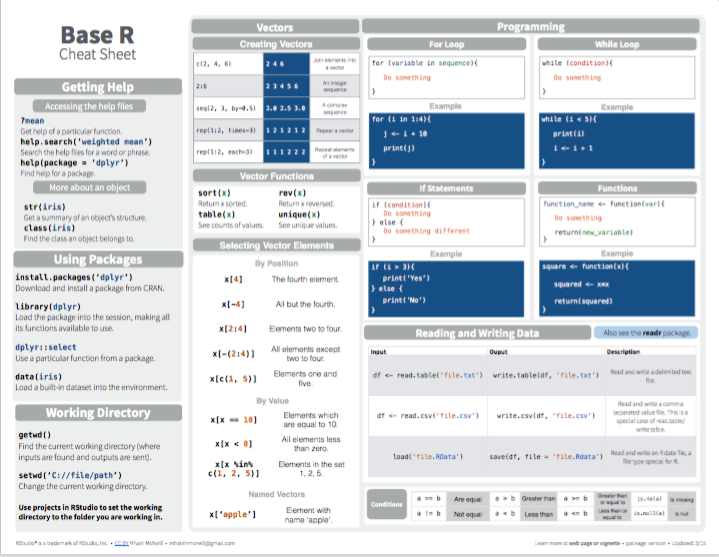
Figure 3.1: Base R summary from Posit cheatsheets.

• More advanced aspects of R:

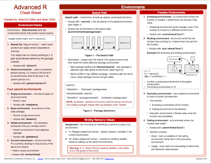
Figure 3.2: Advanced R summary from Posit cheatsheets.

Miscellaneous

Other helpful links that do not fit into the above categories include:

• R-bloggers collects blog posts on R.

• R-exercises provides categorized sets of exercises to help people developing their R programming skills.

• Quick-R (by Robert Kabacoff) is a popular website on R programming.

3.6.3 Preview

We now have a basic understanding of R objects (data vs. functions), and how we can create and examine data by applying functions to data structures.

This chapter concludes Part 1 on the foundations of data science. The upcoming chapters of Part 2 will introduce basic elements of programming in R.

3.7 Exercises

The following questions involve R data structures:

3.7.1 Why and when which data structure?

1. Compare and contrast atomic vectors with lists:

• What are their similarities and differences?
• Under which conditions should we use a list, rather than an atomic vector?

2. Compare and contrast atomic vectors with matrices:

• What are their similarities and differences?
• Under which conditions should we use a matrix, rather than an atomic vector?

3. Compare and contrast lists with data frames:

• What are their similarities and differences?
• Under which conditions should we use a list, rather than a data frame?

3.7.2 List data

In Section 3.4.3, we defined a data frame df to characterize five people as follows:

(df <- data.frame(name, gender, age))
#>     name gender age
#> 1   Adam   male  21
#> 2    Ben   male  19
#> 3 Cecily female  20
#> 4  David   male  48
#> 5 Evelyn   misc  45

• Save the same information as a list ls.

• Show how individual variables (e.g., the age vector) and values (e.g., Cecily’s age) can be accessed in df and ls.

• Why would the data frame be a better choice of data structure here?
  (Hint: Show how the entire information of a person could be accessed in df vs. in ls.)

• Bonus: Can you save the data of df as a list ls_2 in which every element contains all information of each person?
  (Hint: As the information on a person contains different data types, ls_2 must by a list of lists.)

3.7.3 Manipulating matrices

Assuming a matrix mx:

(mx <- matrix(letters[1:4], nrow = 2, ncol = 2, byrow = TRUE))
#>      [,1] [,2]
#> [1,] "a"  "b" 
#> [2,] "c"  "d"

Write R expressions that either apply functions or use some form of indexing to retrieve and replace individual elements for creating the following variants of the matrix mx:

#>      [,1] [,2]
#> [1,] "a"  "b" 
#> [2,] "c"  "d"
#>      [,1] [,2]
#> [1,] "a"  "b" 
#> [2,] "c"  "d"
#>      [,1] [,2]
#> [1,] "a"  "b" 
#> [2,] "c"  "d"
#>      [,1] [,2]
#> [1,] "a"  "b" 
#> [2,] "c"  "d"

# (a)
mx_1  # transpose mx: 
#>      [,1] [,2]
#> [1,] "a"  "c" 
#> [2,] "b"  "d"

# (b)
mx_2  # mirror/swap rows of mx: 
#>      [,1] [,2]
#> [1,] "c"  "d" 
#> [2,] "a"  "b"

# (c)
mx_3  # mirror/swap columns of mx: 
#>      [,1] [,2]
#> [1,] "b"  "a" 
#> [2,] "d"  "c"

# (d)
mx_4  # swap only the elements of the 2nd column of mx: 
#>      [,1] [,2]
#> [1,] "a"  "d" 
#> [2,] "c"  "b"

Hint: This exercise could trivially be solved by creating the matrices mx_1 to mx_4 from scratch. However, the purpose of the exercise is to use indexing for retrieving and replacing matrix elements.

3.7.4 Familiar frames

In Exercise 2.6.3 of Chapter 2 you created vectors to represent information about yourself and (at least four of) your family members.

• Represent the same information in a data frame and then use R to answer the same queries for this data structure.

Hint: As data frames are a list of vectors, these tasks can either be solved by indexing/subsetting a rectangular data structure or by accessing the individual vectors of a data frame.

For additional exercises on R data structures, see Chapter 1: Basic R concepts and commands of the ds4psy textbook (Neth, 2023a):

3.7.5 Survey age

• See 1.8.7 Exercise 7

3.7.6 Exploring participant data

• See 1.8.8 Exercise 8

This concludes our exercises on basic R data structures.

---

18. We occasionally refer to tabular data structures as being “rectangular” or “tables”. This is fine when the context makes it clear that we refer to data frames or tibbles, but has potential for creating confusion. For instance, matrices are rectangular as well, and an R table is a special type of n-dimensional array.↩︎

19. Re-coding continuous variables as categorical variables can be useful, but also results in a loss of information. For this reason, we usually create additional variables in such cases, so that we retain the original values.↩︎