23 Prediction

Prediction is a key goal of modeling, but also a general goal of adaptation and learning.

We aim to develop predictive algorithms (or statistical models) that solve different predictive tasks: A predictive algorithm provides a rule that either (a) predicts a value on some scale, or (b) classifies an entity.

A key component of any predictive enterprise consists in evaluating predictive performance.

Preparation

Recommended background readings for this chapter include:

Chapter 3: Linear Regression of James et al. (2021)
Chapter 4: Classification of James et al. (2021)

Chapter 23: Model basics of the r4ds book (Wickham & Grolemund, 2017).

Preflections

What are the purposes of science?
What is the difference between explanation and prediction?
What is less/more difficult and less/more useful?
What would we like to predict?

23.1 Introduction

Prediction is very difficult, especially if it’s about the future!

Niels Bohr

This familiar quote always sounds a bit funny, although it is not immediately clear why. The fact that the same or highly similar quotes are also attributed to Mark Twain and Yogi Berra suggest that it expresses something obvious — some fact that is widely accessible and agreed upon. And while it may seem circular, it actually is not: Although most predictions may concern the future, we can predict anything unknown, including things that happened in the past. When predicting data, some criterion for measuring the deviation between predicted and true values can be used to evaluate predictions.

The temporal dimension in the quote has an analogue in the type of sampling that is used to evaluate predictions: Predicting different data from an existing sample corresponds to predicting the past, whereas predicting new data (i.e., out-of-sample) corresponds to predicting the future.

The basic principles discussed in this chapter will apply to both general types of prediction.
As we will see, even when predicting the past or data within a given sample, prediction remains difficult.

On of the most fundamental properties of thought is its power of predicting events.

K.J.W. Craik (1943), The nature of explanation, Ch. 5

Clarify key terminology: Prediction.

Distinguish between explanation (understanding, accounting for past data) and prediction (or inference, accounting for novel data).

An ability to predict implies specifying some mechanism. This does not need to be the true underlying mechanism, but some explicit model (which could be the actual mechanism or an as if model).

Key terminology:

informal/verbal vs. formal models
criteria for evaluating predictions
bias-accuracy trade-off in models

Goals of this chapter:

Understanding basic principles, rather than learning particular methods. Building up intuitions behind predictive modeling, rather than emphasizing statistical procedures (like regression modeling, KNN, etc.).

23.2 Essentials of prediction

23.2.1 Explaining vs. predicting

Science ultimately aims for explaining and understanding the underlying mechanisms: Causal interplay of variables (i.e., how a phenomenon comes about).
But before an explanation in this fundamental sense is even conceivable, a more modest goal is to predict outcomes. Being able to predict implies detecting an association (aka. covariation or correlation) between variables. Knowledge that pretends to explain without being able to predict (which actually is quite common by so-called experts, e.g., in biology, medicine, nutrition, finance, or sports) is fake and phony — mere story-telling and useless mumbo-jumbo that may entertain, but must not be taken seriously.

Ubiquitous examples of snake-oil sellers:

Amazing miracle cures: If this remedy really worked, why would big business and the scientific community ignore it?
Financial analysts on investing on the stock market: If the tips and strategies of “financial analysts” actually worked, would they spend their time telling us about it?
Sports experts: So-called tactical “analyses” looks really smart post-hoc, but do they successfully predict the next game’s outcome?

The simple test: Can they successfully predict? If not, all fancy terminology and well-formed phrases is just hot air and BS. Thus, the ability of prediction is the litmus test for useful knowledge, as opposed to self-indulgent speculation.

23.2.2 Examples

Consider the following examples:

The average prediction error of our forecast is below 1%.
This screening test is 99% accurate in detecting some condition.
This algorithm detects fraudulent credit card transactions with an accuracy of 99%.

Note different types of tasks: 1. usually refers to a regression problem, but 2. and 3. to classification tasks.

All three statements sound pretty good, but we should not stop there, but rather ask further questions.

What is the measure on which the test quality is being evaluated and reported? What about other measures?
What is the baseline performance and the performance of alternative algorithms?

Three key questions to ask before trying to predict anything:

Predict what? (Type of task?)
How is performance or predictive success evaluated? (Type of measure?)
What is the baseline performance and the performance of alternative benchmarks?

Distinguish between different prediction tasks and the measures used for evaluating success:

1. Two principle predictive tasks: metric predictions vs. classification tasks
2. Different measures for evaluating (quantifying) the quality of predictions

Note: It is tempting to view classification tasks and quantitative tasks as two types of “qualitative” vs. “quantitative” predictions. However, this would be misleading, as qualitative predictions are also evaluated in a quantitative fashion. Thus, we prefer to distinguish between different tasks, rather than different types of prediction.

23.2.3 Types of tasks

ad 1A: Distinguish between two types of predictive tasks:

quantitative prediction tasks: Point predictions with numeric outcomes. Main goal: Predict some value on a scale.
Secondary goal: Evaluation by the distance between predicted and true values.
qualitative prediction tasks: Classification tasks. Main goal: Predict the membership in some category.
Secondary goal: Evaluation by a 2x2 matrix of predicted vs. true cases (with 2 correct cases and 2 errors).

Notes:

James et al. (2021) distinguish between regression tasks and classification tasks. As we can use regression models for solving classification tasks, we prefer the distinction between quantitative and qualitative predictions.
Some authors (e.g., in 7 Fitting models with parsnip of Tidy Modeling with R) distinguish between different modes. The mode reflects the type of prediction outcome. For numeric outcomes, the mode is regression; for qualitative outcomes, it is classification.

23.2.4 Evaluating predictive success

ad 1B: Given some prediction, how is predictive success evaluated (quantified)?

Remember the earlier example of the mammography problem: Screening has high sensitivity and specificity, but low PPV.

Note that — for all types of prediction — there are always trade-offs between many alternative measures for quantifying their success. Maximizing only one of them can be dangerous and misleading.

23.2.5 Baseline performance and other benchmarks

ad 2. On first glance, the instruction “Predict the phenomenon of interest with high accuracy.” seems a reasonable answer to the question “What characterizes a successful predictive algorithm?”.
However, high accuracy is not very impressive if the baseline is already quite high. For instance, if it rains on only 10% of all summer days in some region, always predicing “no rain” will achieve an accuracy of 90%.

This seems trivial, but consider the above examples of detecting some medical condition or fraudulent credit card transactions: For a rare medical condition, a fake pseudo-test that always says “healthy” would achieve an impressive accuracy. Similarly, if over 99% of all credit card transactions are legitimate, always predicting “transaction is ok” would achieve an accuracy of over 99%…

Hence, we should always ask ourselves:

What is the lowest possible benchmark (e.g., for random predictions)?
What levels can be achieved by naive or very simple predictions?

As perfection is typically impossible, we need to decide how much better our rule needs to be than alternative algorithms. For this latter evaluation, it is important to know the competition.

23.3 Quantitative prediction tasks

Forecasting some probability vs. predicting values by some model (e.g., linear regression model).

Goal: Predicting some value (on a scale).

Method: Linear regression.

Disclaimer

Note that this section is still unfinished.

23.3.1 Introduction

This section provides a gentle introduction to linear regression models. Rather than providing a statistical treatment — which typically uses the simple LR model to transition into the realms of multiple predictors, different types of variables and their possible transformations, and non-linear extensions in the GLM framework — we aim to illustrate the principles behind linear regression and key intuitions that are important for any kind of statistical modeling.

Specific goals:

Understand the relation between correlation and simple linear regression models
Understand common measures to assess model accuracy
Understand different elements and uses of a model
Understand the difference between explaining existing (model fitting) data and predicting new data

Example:
Using historic data by Galton (Friendly, 2023) from first correlation and “regression”:

# install.packages("HistData")
library(HistData)

# ?GaltonFamilies  
dim(GaltonFamilies)  # 934 x 8
#> [1] 934   8
# as_tibble(GaltonFamilies)
# View(GaltonFamilies)

GF <- tibble::as_tibble(GaltonFamilies)


# Note: The more limited dataset Galton contains 
#       abstracted/processed data of 928 parent/child pairs.
# dim(Galton)

Goal: Study the relationship of height between generations, specifically: Association between parent’s and children’s height.

Note: We are tempted to interpret this as causal (i.e., parent’s height as a cause, children’s height as an effect). However, if a relationship exists, we can also view it from the opposite direction: To what extent can parent’s height be predicted by children’s height?

The variable midparentHeight is a weighted average of father and mother, with values of mother multiplied by a factor of 1.08. To account for the fact that men are on average taller than women, Galton “transmuted” (Galton, 1886, p. 247) women into men (see Hanley, 2004, for details). We can verify the calculation of midparentHeight and see the effects of this manipulation by comparing the histograms for all three variables:

# Verify definition of midparentHeight:
mpH <- (GF$father + (1.08 * GF$mother))/2
all.equal(GF$midparentHeight, mpH)
#> [1] TRUE

# Compare histograms of 3 distributions:
ggplot(GF) + 
  geom_histogram(aes(x = midparentHeight), fill = "grey67", binwidth = 1) + 
  geom_histogram(aes(x = father), fill = "deepskyblue", alpha = .50, binwidth = 1) + 
  geom_histogram(aes(x = mother), fill = "deeppink", alpha = .50, binwidth = 1) + 
  labs(title = "Distribution of height values (for fathers, mothers, vs. midparents)",
       x = "Height (in inches)", y = "Frequency count", 
       caption = "[Data from HistData::GaltonFamilies]") + 
  theme_ds4psy()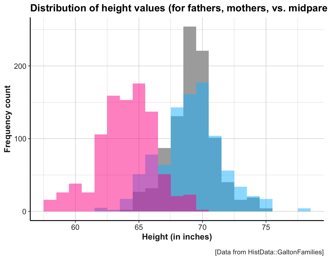

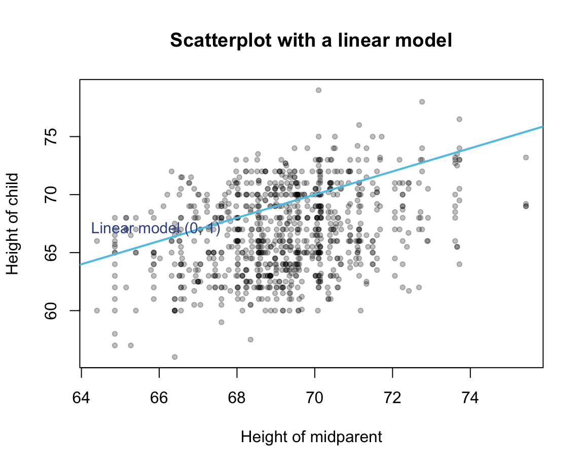
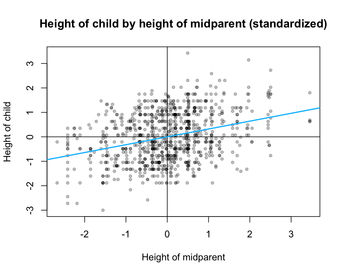
Scatterplot of raw values of childHeight as a function of midparentHeight:

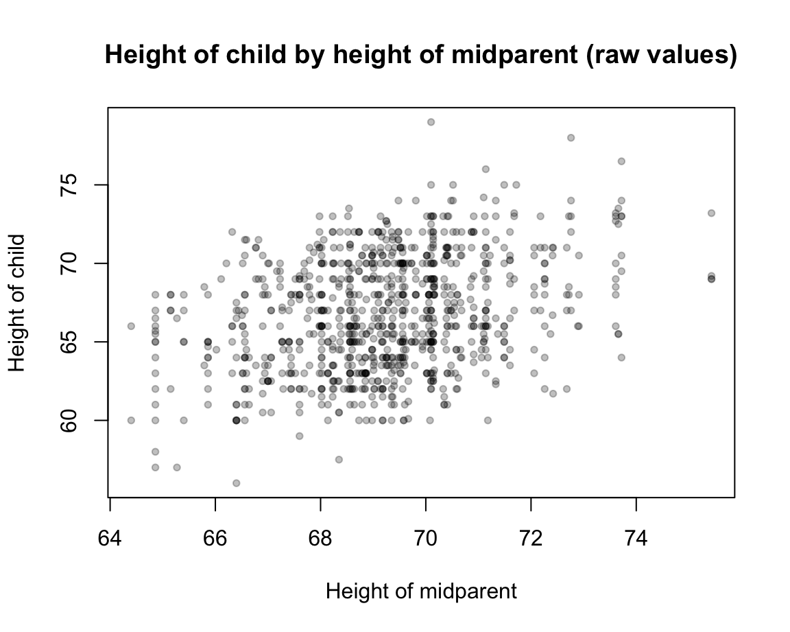
Specific task: Explain or predict the values of childHeight by values of midparentHeight.

23.3.2 A basic model

We want to predict the true values of childHeight $y_i$.
What would the most simple model be? A null-model for this data: Predict the mean criterion value $\hat{y_i}$ for all data points $x_i$: For all values of $x_i$, predict $\bar{y_i} = \sum_{i=1}^{n}{y_i}$. Graphically, this basic model is a horizontal line with a $y$-intercept given by the mean criterion value:

#> [1] 69.20677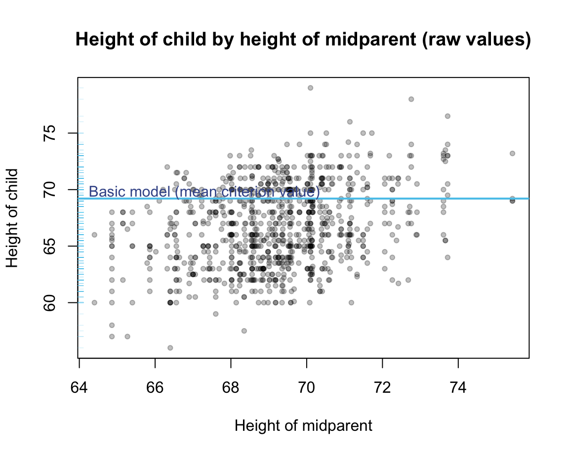

Predicting the mean criterion value $\bar{y_i}$ for all possible data points $x_i$ provides a veritable model. Although this model is primitive and inflexible, it is very simple, as it employs only one parameter (i.e., the $y$-intercept of the mean). Nonetheless, it makes a specific prediction for any old or new data point, albeit the rather boring prediction of the same value.

How good is this model? We typically evaluate models by the accuracy of their predictions. Given some true criterion values, we can measure model accuracy by quantifying the deviations between these true values $\hat{y_i}$ and the corresponding predicted values $\hat{y_i}$.

Illustration of some deviations between true criterion values and model values (for a random sample of 10 data points):

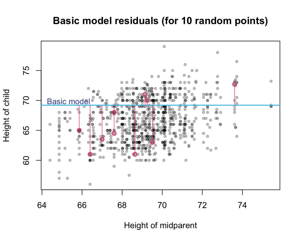
As deviations are computed from differences (i.e., true value $y_i$ minus predicted value $\bar{y_i}$) that can be positive or negative, they are typically squared (so that all differences are positive and larger differences weigh more than smaller ones) and summed (over all data points). Thus, the accuracy of our basic model or the amount of deviation between true data values and the model predictions can be quantified as the total sum of squares (TSS):

\[\text{TSS} = \sum_{i=1}^{n}{(y_i - \bar{y_i})^2}\]

As the value of TSS increases with larger deviations between true and predicted data values, smaller values of TSS indicate better models (i.e., ideally, $\text{TSS} \rightarrow 0$). We can express this in R as follows:

# Measures of model accuracy: 
# (see @JamesEtAl2021, p. 69ff.): 

# Total sum of squares (TSS): ---- 
TSS <- function(true_vals, pred_vals = NA){
  
  # Special case: 
  if (is.na(pred_vals)){
    pred_vals <- mean(true_vals)
  }
  
  sum((true_vals - pred_vals)^2)
}

and then compute the accuracy of our basic model as:

TSS(true_vals = GF$midparentHeight)
#> [1] 3030.886

Thus, the accuracy of our model is measured to be 3030.89. This is definitely not close to our ideal of a deviation value of zero ($\text{TSS} \rightarrow 0$). So can we find better models?

As TSS is our first measure of model accuracy, it is important to understand the role of such measures: As the fit between data and model predictions is expressed as a numeric value, we can vary aspects of the model to see whether this improves or decreases the quality of our model (as quantified by this particular measure).

When changing models, we need to distinguish between two aspects:

varying parameters within a given model type: Changing the value of parameter(s) given by the current model type to optimize the fit of a given model type; vs.
varying model types: Changing to a different model type (with different numbers or types of parameters).

As our basic model contains only one parameter (the $y$-intercept), we could try to predict different values (i.e., different variants of the same model type) and compare the accuracy of these alternative models to the one of our basic model:

TSS(true_vals = GF$midparentHeight, pred_vals = 66)
#> [1] 12635.58
TSS(true_vals = GF$midparentHeight, pred_vals = 68)
#> [1] 4391.072
TSS(true_vals = GF$midparentHeight, pred_vals = 70)
#> [1] 3618.568

We see that other predictions do not improve further on our basic model (given this measure and model type). Given the nature of our model and our measure, using the mean value as our only model parameter optimizes this particular accuracy measure, i.e., provides the best model when accepting the measure (TSS) and the constraints of our model type (i.e., it being a horizontal line).

23.3.3 Linear models

How can we improve on this basic model?

A more powerful model family: Create linear models with 2 parameters: intercept and slope.

\[\begin{align} y & = a + bx\\ & = b_0 + b_1 x \end{align}\]

Generate many random models: Each model generates “predictions” for criterion values.

Example: $y = 0 + 1 x$

Quantify the deviation of the model predictions from the corresponding data point (truth).

Goal: Optimize the model by minimizing their accuracy/deviation measure.

Model accuracy

To optimize, we need a measure to quantify model accuracy:

For linear models, a basic accuracy measure follows the logic of quantifying the amount of deviation between true and predicted values. This deviation is given by computing the so-called residuals (i.e., the difference between true values $y_i$ and predicted values $\hat{y_i}$).

Illustration of residual values (for a random sample of 10 data points):

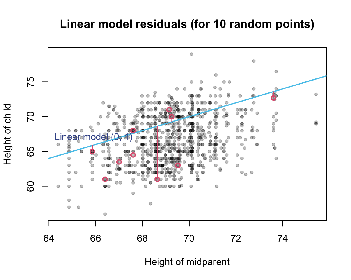
Again, residual values exist for every point, can be positive or negative: squaring them, and adding the resulting sums. The resulting accuracy measure is known as the residual sums of squares (RSS, see James et al., 2021, p. 69):

\[\text{RSS} = \sum_{i=1}^{n}{(y_i - \hat{y_i})^2}\]

Note that TSS (above) is but a special case of RSS (with predicting a single value $\bar{y_i}$ for all values of $x_i$, rather than predicting different values of $y_i$ for different values of $x_i$) and that RSS will later be used to compute the residual square error (RSE) and combined with TSS to obtain the $R^2$-measure.

Again, we can easily define an R function for the residual sum of squares (RSS), when providing both the true and predicted values as arguments:

# Measures of model accuracy: 
# (see @JamesEtAl2021, p. 69ff.): 

# Residual sum of squares (RSS): ---- 
RSS <- function(true_vals, pred_vals){
  
  sum((true_vals - pred_vals)^2)
}

Compute RSS for various models…

A more systematic approach: Rather than randomly generating parameters and assessing the fit of the corresponding model to the data, we could ask: What would be good values for intercept and slope?

Intercept value is arbitrary in the sense that it depends on the scale of the criterion. If the criterion was standardized, the intercept could be zero.

Slope represents the linear association between the single predictor and the criterion variable.

Correlation

Just as there are multiple ways to measure the central tendency of a distribution of values (e.g., mean, median, mode) there are many measures of the degree of association between variables. The appropriate measure depends on the variables’ scales (e.g., continuous vs. categorical variables) and the mathematical way of computing the degree of association (e.g., how are prediction errors quantified).

Covariation:

Formula (as variance between two variables $X$ and $Y$):

\[s_{XY} = \frac{1}{N} \sum_{m=1}^{n}(x_m - \bar{x}) \cdot (y_m - \bar{y})\]

As an R function:

my_cov <- function(N, x, y){
  
  mn_x <- mean(x)
  mn_y <- mean(y)
  
  1/N * sum((x - mn_x) * (y - mn_y))
  
}

# Example:
my_cov(N = nrow(GF), x = GF$midparentHeight, y = GF$childHeight)
#> [1] 2.068275

A common measure of linear association: Pearson correlation (aka. Bravais correlation, product moment correlation, or just correlation):

Mathematically, the measure of covariation is normalized by standard deviations:

\[r_{XY} = \frac{1}{N} \sum_{m=1}^{n} \frac{(x_m - \bar{x})}{s_X} \cdot \frac{(y_m - \bar{y})}{s_Y}\]

Viewing as $z$-transformed variables or as the covariation (from above) normalized by the product of the variables’ standard deviations:

\[r_{XY} = \frac{1}{N} \sum_{m=1}^{n} (z_{x_m} \cdot z_{y_m}) = \frac{ S_{XY}}{S_X \cdot S_Y}\]

As an R function:

my_cor <- function(N, x, y){
 
  my_cov(N, x, y)/(sd(x) * sd(y))
   
}

# Example:
my_cor(N = nrow(GF), x = GF$midparentHeight, y = GF$childHeight)
#> [1] 0.3206063

Using the R stats function cor():

(cor_1 <- stats::cor(x = GF$midparentHeight, y = GF$childHeight, method = "pearson"))
#> [1] 0.3209499

Note a slight numerical difference: The stats function cor(method = "pearson") divides the covariation by $N - 1$:

cor_1
#> [1] 0.3209499
my_cor(N = (nrow(GF) - 1), x = GF$midparentHeight, y = GF$childHeight)
#> [1] 0.3209499

The correlation value $r_{XY}$ has a range from $-1$ to $+1$, with typical evaluations:

$|r_{XY}| \approx .10$: weak association
$|r_{XY}| \approx .30$: moderate association
$|r_{XY}| \geq .50$: strong association

Measures of association for ordinal variables include Kendalls $\tau$ and Spearmans rank correlation $r_S$. In R, they can be accessed by providing corresponding method arguments to the cor() function.

For binomial or categorical variables, a number of association measures exist (including the $\phi$ coefficient, Yules $Q$, the odds ratio $OR$, $\chi$^2, or Cramér’s $V$).

Linear regression

Linear regression model:

# Linear regression model (raw values):
lr_1 <- lm(childHeight ~ midparentHeight, data = GF)

summary(lr_1)
#> 
#> Call:
#> lm(formula = childHeight ~ midparentHeight, data = GF)
#> 
#> Residuals:
#>     Min      1Q  Median      3Q     Max 
#> -8.9570 -2.6989 -0.2155  2.7961 11.6848 
#> 
#> Coefficients:
#>                 Estimate Std. Error t value Pr(>|t|)    
#> (Intercept)     22.63624    4.26511   5.307 1.39e-07 ***
#> midparentHeight  0.63736    0.06161  10.345  < 2e-16 ***
#> ---
#> Signif. codes:  0 '***' 0.001 '**' 0.01 '*' 0.05 '.' 0.1 ' ' 1
#> 
#> Residual standard error: 3.392 on 932 degrees of freedom
#> Multiple R-squared:  0.103,  Adjusted R-squared:  0.102 
#> F-statistic:   107 on 1 and 932 DF,  p-value: < 2.2e-16

plot(x = GF$midparentHeight, y = GF$childHeight, 
     pch = 20, col = adjustcolor("black", .25), 
     main = "Height of child by height of midparent (raw values)",
     xlab = "Height of midparent", ylab = "Height of child")

# Plot linear regression line:
abline(lr_1, col = "deepskyblue", lwd = 2)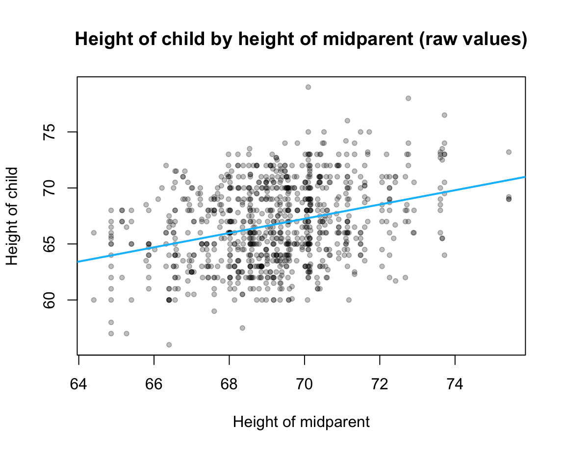

Interpretation:

Interpreting model coefficients:

Intercept: Can be difficult to interpret, as predictor values of zero often (and here) make no sense. Important to understand that it determines the overall height of the regression line and that it is expressed in units of the predictor variable $Y$.
Coefficient of predictor: Indicates the amount of association between this predictor and the criterion, given any other predictors. Value depends on scale and is hard to interpret unless variables were standardized (see below). Importantly, we need to consider value and its SE. If value differs more than 2 SEs from 0, it is significant (unlikely that the observed effect is due to chance alone).

As above, we can quantify model accuracy by measuring the deviation of our predicted values (on the linear regression curve) from the true values by RSS:

# Compute model predictions (from model coefficients):
lr_1_predictions <- coefficients(lr_1)[1] + (coefficients(lr_1)[2] * GF$midparentHeight)

# Note: Model predictions are also provided by lr_1$fitted.values:  
all.equal(lr_1_predictions, lr_1$fitted.values, check.attributes = FALSE)
#> [1] TRUE

RSS(true_vals = GF$childHeight, pred_vals = lr_1_predictions)
#> [1] 10721.47

Note that RSS value is much lower (i.e., better) than the RSS (or TSS) value of our basic model. (Below, we will use the difference between RSS and TSS to compute a key measure of model accuracy known as the $R^2$-statistic.)

The values of RSE, $R^2$ and $F$-statistic in the summary() provide overall measures of model accuracy or quality (and will be defined and explained below).

Standardizing model variables

Standardizing model variables (both criterion and predictor) with the scale() function:

# z-Standardization:
z_childHeight <- scale(GF$childHeight)

# Histogram: 
hist(z_childHeight, col = "grey90", border = "white")

# Show mean value and +/- 1 SD:
abline(v = mean(z_childHeight), col = "deeppink", lwd = 2, lty = 1)
abline(v = mean(z_childHeight) - sd(z_childHeight), col = "deepskyblue", lwd = 1, lty = 2)
abline(v = mean(z_childHeight) + sd(z_childHeight), col = "deepskyblue", lwd = 1, lty = 2)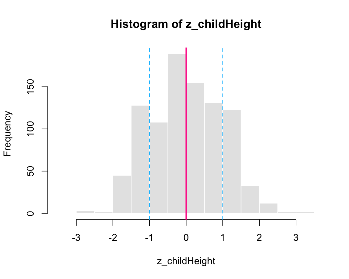


z_midparentHeight <- scale(GF$midparentHeight)

Standardized model (both criterion and predictor):

# Linear regression model (standardized):
lr_2 <- lm(scale(childHeight) ~ scale(midparentHeight), data = GF)

summary(lr_2)
#> 
#> Call:
#> lm(formula = scale(childHeight) ~ scale(midparentHeight), data = GF)
#> 
#> Residuals:
#>     Min      1Q  Median      3Q     Max 
#> -2.5025 -0.7540 -0.0602  0.7812  3.2646 
#> 
#> Coefficients:
#>                         Estimate Std. Error t value Pr(>|t|)    
#> (Intercept)            7.570e-16  3.101e-02    0.00        1    
#> scale(midparentHeight) 3.209e-01  3.102e-02   10.35   <2e-16 ***
#> ---
#> Signif. codes:  0 '***' 0.001 '**' 0.01 '*' 0.05 '.' 0.1 ' ' 1
#> 
#> Residual standard error: 0.9476 on 932 degrees of freedom
#> Multiple R-squared:  0.103,  Adjusted R-squared:  0.102 
#> F-statistic:   107 on 1 and 932 DF,  p-value: < 2.2e-16

Interpretation:

Standardizing the predictor and criterion variables changes their scale and facilitates the interpretation of the coefficients. Importantly, we now need to interpret values in units of standard deviations.

In the $z$-standardized model lr_2, the intercept value is (near) zero and the regression coefficient of the linear predictor corresponds to the Pearson correlation cor_1 (computed above):

near(coefficients(lr_2)[1], 0)
#> (Intercept) 
#>        TRUE
near(coefficients(lr_2)[2], cor_1)
#> scale(midparentHeight) 
#>                   TRUE

By comparing the summary() outputs for both models, we see that the model’s residual standard error (RSE) changes when rescaling the criterion variable. However, $R^2$ and $F$-statistic are unchanged by the standardization from lr_1 to lr_2.

Key elements of a model

summary(lr_1)
#> 
#> Call:
#> lm(formula = childHeight ~ midparentHeight, data = GF)
#> 
#> Residuals:
#>     Min      1Q  Median      3Q     Max 
#> -8.9570 -2.6989 -0.2155  2.7961 11.6848 
#> 
#> Coefficients:
#>                 Estimate Std. Error t value Pr(>|t|)    
#> (Intercept)     22.63624    4.26511   5.307 1.39e-07 ***
#> midparentHeight  0.63736    0.06161  10.345  < 2e-16 ***
#> ---
#> Signif. codes:  0 '***' 0.001 '**' 0.01 '*' 0.05 '.' 0.1 ' ' 1
#> 
#> Residual standard error: 3.392 on 932 degrees of freedom
#> Multiple R-squared:  0.103,  Adjusted R-squared:  0.102 
#> F-statistic:   107 on 1 and 932 DF,  p-value: < 2.2e-16

# Note: 
# str(lr_1)  # shows list structure with 12 elements

# Important elements: ------ 
coefficients(lr_1)
#>     (Intercept) midparentHeight 
#>      22.6362405       0.6373609
lr_1$coefficients
#>     (Intercept) midparentHeight 
#>      22.6362405       0.6373609

# Different types of values: ----- 

# in data:
GF$midparentHeight  # predictor values
#>  [1] 75.43 75.43 75.43 75.43 73.66 73.66 73.66 73.66 72.06 72.06 72.06 72.06
#> [13] 72.06 72.06 72.06 69.09 69.09 69.09 69.09 69.09 69.09 73.72 73.72 73.72
#> [25] 73.72 73.72 73.72 73.72 72.91 72.91 72.91 72.89 72.37 70.48 70.48 70.48
#> [37] 70.48 70.48 70.48 70.48 70.48 69.94 72.68 72.68 72.68 72.68 72.41 72.41
#> [49] 72.41 71.60 71.60 71.60 71.60 71.60 71.60 71.60 71.60 71.60 71.33 71.33
#> [61] 71.33 71.33 71.33 71.33 71.06 71.06 71.06 70.62 73.61 73.61 73.61 73.61
#> [73] 73.61 73.61 73.61
#>  [ reached getOption("max.print") -- omitted 859 entries ]
GF$childHeight      # criterion values
#>  [1] 73.2 69.2 69.0 69.0 73.5 72.5 65.5 65.5 71.0 68.0 70.5 68.5 67.0 64.5 63.0
#> [16] 72.0 69.0 68.0 66.5 62.5 62.5 69.5 76.5 74.0 73.0 73.0 70.5 64.0 70.5 68.0
#> [31] 66.0 66.0 65.5 74.0 70.0 68.0 67.0 67.0 66.0 63.5 63.0 65.0 71.0 62.0 68.0
#> [46] 67.0 71.0 70.5 66.7 72.0 70.5 70.2 70.2 69.2 68.7 66.5 64.5 63.5 74.0 73.0
#> [61] 71.5 62.5 66.5 62.3 66.0 64.5 64.0 62.7 73.2 73.0 72.7 70.0 69.0 68.5 68.0
#>  [ reached getOption("max.print") -- omitted 859 entries ]

# in model:
lr_1$fitted.values
#>        1        2        3        4        5        6        7        8 
#> 70.71237 70.71237 70.71237 70.71237 69.58424 69.58424 69.58424 69.58424 
#>        9       10       11       12       13       14       15       16 
#> 68.56447 68.56447 68.56447 68.56447 68.56447 68.56447 68.56447 66.67150 
#>       17       18       19       20       21       22       23       24 
#> 66.67150 66.67150 66.67150 66.67150 66.67150 69.62249 69.62249 69.62249 
#>       25       26       27       28       29       30       31       32 
#> 69.62249 69.62249 69.62249 69.62249 69.10622 69.10622 69.10622 69.09348 
#>       33       34       35       36       37       38       39       40 
#> 68.76205 67.55744 67.55744 67.55744 67.55744 67.55744 67.55744 67.55744 
#>       41       42       43       44       45       46       47       48 
#> 67.55744 67.21326 68.95963 68.95963 68.95963 68.95963 68.78754 68.78754 
#>       49       50       51       52       53       54       55       56 
#> 68.78754 68.27128 68.27128 68.27128 68.27128 68.27128 68.27128 68.27128 
#>       57       58       59       60       61       62       63       64 
#> 68.27128 68.27128 68.09919 68.09919 68.09919 68.09919 68.09919 68.09919 
#>       65       66       67       68       69       70       71       72 
#> 67.92711 67.92711 67.92711 67.64667 69.55238 69.55238 69.55238 69.55238 
#>       73       74       75 
#> 69.55238 69.55238 69.55238 
#>  [ reached getOption("max.print") -- omitted 859 entries ]
lr_1$residuals
#>           1           2           3           4           5           6 
#>  2.48762699 -1.51237301 -1.71237301 -1.71237301  3.91575578  2.91575578 
#>           7           8           9          10          11          12 
#> -4.08424422 -4.08424422  2.43553321 -0.56446679  1.93553321 -0.06446679 
#>          13          14          15          16          17          18 
#> -1.56446679 -4.06446679 -5.56446679  5.32849508  2.32849508  1.32849508 
#>          19          20          21          22          23          24 
#> -0.17150492 -4.17150492 -4.17150492 -0.12248587  6.87751413  4.37751413 
#>          25          26          27          28          29          30 
#>  3.37751413  3.37751413  0.87751413 -5.62248587  1.39377645 -1.10622355 
#>          31          32          33          34          35          36 
#> -3.10622355 -3.09347633 -3.26204866  6.44256343  2.44256343  0.44256343 
#>          37          38          39          40          41          42 
#> -0.55743657 -0.55743657 -1.55743657 -4.05743657 -4.55743657 -2.21326168 
#>          43          44          45          46          47          48 
#>  2.04036946 -6.95963054 -0.95963054 -1.95963054  2.21245690  1.71245690 
#>          49          50          51          52          53          54 
#> -2.08754310  3.72871923  2.22871923  1.92871923  1.92871923  0.92871923 
#>          55          56          57          58          59          60 
#>  0.42871923 -1.77128077 -3.77128077 -4.77128077  5.90080667  4.90080667 
#>          61          62          63          64          65          66 
#>  3.40080667 -5.59919333 -1.59919333 -5.79919333 -1.92710589 -3.42710589 
#>          67          68          69          70          71          72 
#> -3.92710589 -4.94666709  3.64762382  3.44762382  3.14762382  0.44762382 
#>          73          74          75 
#> -0.55237618 -1.05237618 -1.55237618 
#>  [ reached getOption("max.print") -- omitted 859 entries ]

# Note: 
# (1) The fitted.values are equal to the predicted criterion values, given 
#     the raw values of the predictor and the model (coefficients):
model_predictions <- lr_1$coefficients[1] + lr_1$coefficients[2] * GF$midparentHeight
all.equal(model_predictions, lr_1$fitted.values, check.attributes = FALSE)
#> [1] TRUE

# (2) The residuals are equal to raw values (of criterion) minus fitted.values: 
model_errors <- GF$childHeight - lr_1$fitted.values
all.equal(model_errors, lr_1$residuals)
#> [1] TRUE

Fitting vs. predicting

Fitting a model on an entire dataset does not really “predict” anything. Instead, we fit a linear model to data for constructing a simple (model-based) explanation of the dataset.

The model’s “predictions” are its fitted values:

# The predict() function uses a model to generate predictions: ------ 

predict(object = lr_1)  # with data used to fit the model: fitted.values == predicted values
#>        1        2        3        4        5        6        7        8 
#> 70.71237 70.71237 70.71237 70.71237 69.58424 69.58424 69.58424 69.58424 
#>        9       10       11       12       13       14       15       16 
#> 68.56447 68.56447 68.56447 68.56447 68.56447 68.56447 68.56447 66.67150 
#>       17       18       19       20       21       22       23       24 
#> 66.67150 66.67150 66.67150 66.67150 66.67150 69.62249 69.62249 69.62249 
#>       25       26       27       28       29       30       31       32 
#> 69.62249 69.62249 69.62249 69.62249 69.10622 69.10622 69.10622 69.09348 
#>       33       34       35       36       37       38       39       40 
#> 68.76205 67.55744 67.55744 67.55744 67.55744 67.55744 67.55744 67.55744 
#>       41       42       43       44       45       46       47       48 
#> 67.55744 67.21326 68.95963 68.95963 68.95963 68.95963 68.78754 68.78754 
#>       49       50       51       52       53       54       55       56 
#> 68.78754 68.27128 68.27128 68.27128 68.27128 68.27128 68.27128 68.27128 
#>       57       58       59       60       61       62       63       64 
#> 68.27128 68.27128 68.09919 68.09919 68.09919 68.09919 68.09919 68.09919 
#>       65       66       67       68       69       70       71       72 
#> 67.92711 67.92711 67.92711 67.64667 69.55238 69.55238 69.55238 69.55238 
#>       73       74       75 
#> 69.55238 69.55238 69.55238 
#>  [ reached getOption("max.print") -- omitted 859 entries ]

We can, however, also use a model for genuine predictions or predicting criterion values for new data values (i.e., predictor values not used for model fitting). To do so, the predict() function receives both a model and new data values (as the object and newdata arguments, respectively):

# Using model to predict criterion values for new data (predictor values):
(my_heights <- seq(50, 80, by = 5))
#> [1] 50 55 60 65 70 75 80
predict(object = lr_1, newdata = data.frame(midparentHeight = my_heights))
#>        1        2        3        4        5        6        7 
#> 54.50429 57.69109 60.87789 64.06470 67.25150 70.43831 73.62511

Note that the newdata argument requires a data frame with the same variable names as those used as predictors in the model.

To illustrate the difference between explaining existing data and genuinely predicting new data, we can split our data into two parts:

GF_train contains $p = 50$% of the observations (rows) of GF;
GF_test contains the other $(1 - p) = 50$% of the observations (rows) of GF.

We use the sample() function to draw a random subset of rows from GF and then numerical indexing on GF to extract two equally sized subsets:

# Sample 50% of 1:nrow(GF) without replacement:
N <- nrow(GF)
set.seed(246)  # reproducible randomness
ix_train <- sort(sample(x = 1:N, size = N/2, replace = FALSE))

# Split data GF into 2 complementary subsets: 
GF_train <- GF[ ix_train, ]
GF_test  <- GF[-ix_train, ]

# Check subsets sizes:
dim(GF_train)  # 467 x 8
#> [1] 467   8
dim(GF_test)   # 467 x 8
#> [1] 467   8

Construct a model by fitting a simple LR to GF_train:

# Linear regression model (unstandardized):
lr_3 <- lm(childHeight ~ midparentHeight, data = GF_train)
summary(lr_3)
#> 
#> Call:
#> lm(formula = childHeight ~ midparentHeight, data = GF_train)
#> 
#> Residuals:
#>    Min     1Q Median     3Q    Max 
#> -8.311 -2.778 -0.100  2.856 11.375 
#> 
#> Coefficients:
#>                 Estimate Std. Error t value Pr(>|t|)    
#> (Intercept)     23.12173    6.43589   3.593 0.000362 ***
#> midparentHeight  0.63486    0.09292   6.832 2.63e-11 ***
#> ---
#> Signif. codes:  0 '***' 0.001 '**' 0.01 '*' 0.05 '.' 0.1 ' ' 1
#> 
#> Residual standard error: 3.481 on 465 degrees of freedom
#> Multiple R-squared:  0.09123,    Adjusted R-squared:  0.08928 
#> F-statistic: 46.68 on 1 and 465 DF,  p-value: 2.629e-11

# Alternative direction: ------ 

# Linear regression model (unstandardized):
lr_3b <- lm(childHeight ~ midparentHeight, data = GF_test)
summary(lr_3b)
#> 
#> Call:
#> lm(formula = childHeight ~ midparentHeight, data = GF_test)
#> 
#> Residuals:
#>    Min     1Q Median     3Q    Max 
#> -8.656 -2.561 -0.276  2.610  9.316 
#> 
#> Coefficients:
#>                 Estimate Std. Error t value Pr(>|t|)    
#> (Intercept)     22.59630    5.62405   4.018 6.85e-05 ***
#> midparentHeight  0.63342    0.08127   7.794 4.30e-14 ***
#> ---
#> Signif. codes:  0 '***' 0.001 '**' 0.01 '*' 0.05 '.' 0.1 ' ' 1
#> 
#> Residual standard error: 3.278 on 465 degrees of freedom
#> Multiple R-squared:  0.1155, Adjusted R-squared:  0.1136 
#> F-statistic: 60.74 on 1 and 465 DF,  p-value: 4.298e-14

Using the model lr_3 for predicting criterion values in GF_test data:

GF_test_predictions <- predict(lr_3, newdata = GF_test)

Evaluating the accuracy of model predictions

The accuracy of linear regression models is typically evaluated by two measures that are based on the TSS and RSS measures from above (see James et al., 2021, p. 69ff., for details):

The residual standard error (RSE) estimates the standard deviation of the irreducible error $\epsilon$ to quantify the extent to which our predictions would miss on average if we knew the true LR line (i.e., the population values $\beta_0$ and $\beta_1$).

The residual standard error (RSE) is based on the residual sums of squares (RSS, see above and James et al., 2021, p. 69):

\[\text{RSS} = \sum_{i=1}^{n}{(y_i - \hat{y_i})^2}\]

and

\[\text{RSE} = \sqrt{\frac{1}{n-2} \cdot \text{RSS}}\]

As RSE quantifies the lack of fit of a model in units of $Y$, lower values are better (ideally, $RSE \rightarrow 0$).

The proportion of variance explained ($R^2$): Whereas RSE provides an absolute measure of model fit (in units of the criterion $Y$), the $R^2$ statistic provides an alternative measure of fit as the proportion of non-erroreous squared deviations, or the proportion of variance explained:

\[R^2 = \frac{\text{TSS} - \text{RSS}}{\text{TSS}}\]

with TSS defined as (see above):

\[\text{TSS} = \sum_{i=1}^{n}{(y_i - \bar{y_i})^2}\]

In contrast to error measures, $R^2$ ranges from $0$ to $1$, with higher values indicating better model fits (ideally, $R^2 \rightarrow 1$).

We can easily define R functions for the residual sum of squares (RSS), the residual standard error (RSE), and the $R^2$-statistic, when providing both the true and predicted values as arguments:

# Measures of model accuracy: 
# (see @JamesEtAl2021, p. 69ff.): 

# Residual standard error (RSE): ----
RSE <- function(true_vals, pred_vals){
  
  n <- length(true_vals)  
  
  rss <- RSS(true_vals, pred_vals)  # defined above
  
  sqrt(1/(n - 2) * rss)
}


# R^2 statistic: ----
Rsq <- function(true_vals, pred_vals){
  
  tss <- TSS(true_vals)  # defined above
  
  rss <- RSS(true_vals, pred_vals)  # defined above
  
  (tss - rss)/tss
}

Checking the accuracy of the original model lr_1:

RSE(true_vals = GF$childHeight, pred_vals = lr_1$fitted.values)
#> [1] 3.391713
Rsq(true_vals = GF$childHeight, pred_vals = lr_1$fitted.values)
#> [1] 0.1030088
# summary(lr_1)  # contains the same values

Comparing to the accuracy of the standardized model lr_2:

RSE(true_vals = scale(GF$childHeight), pred_vals = lr_2$fitted.values)
#> [1] 0.9476041
Rsq(true_vals = scale(GF$childHeight), pred_vals = lr_2$fitted.values)
#> [1] 0.1030088
# summary(lr_2)  # contains the same values

We see that the residual standar error (RSE) changes by re-scaling the criterion, but $R^2$ and $F$-statistic remain the same.

Checking the accuracy of the model lr_3 (fitted to the GF_train subset):

# True vs. predicted values (training data):
true_train_vals <- GF_train$childHeight 
true_pred_vals  <- lr_3$fitted.values

# Model accuracy:
RSE(true_train_vals, true_pred_vals)
#> [1] 3.481212
Rsq(true_train_vals, true_pred_vals)
#> [1] 0.09122942
# summary(lr_3)

+++ here now +++

Next: Checking prediction accuracy for unseen TEST data GF_test…

Distinguish:

explaining old data vs. predicting new data

ToDo:

Next steps:

Elements of a model (e.g., str())
Fitting vs. predicting (explaining old vs. predicting new data)
Regression to the mean (Galton’s discovery/point)
Comparing models (ANOVA)
Multiple predictors (collinearity?)

23.3.4 Comparing models

Using the GaltonFamilies (GF) data, we can try alternative predictors:

Rather than using the complex variable midparentHeight as our predictor, we can compare and contrast regressions using either father or mother as a single predictor (using standardized models):

# Using data from GF: 

# Above, we computed:
# (0) Linear regression model on midparentHeight (standardized):
summary(lr_2)
#> 
#> Call:
#> lm(formula = scale(childHeight) ~ scale(midparentHeight), data = GF)
#> 
#> Residuals:
#>     Min      1Q  Median      3Q     Max 
#> -2.5025 -0.7540 -0.0602  0.7812  3.2646 
#> 
#> Coefficients:
#>                         Estimate Std. Error t value Pr(>|t|)    
#> (Intercept)            7.570e-16  3.101e-02    0.00        1    
#> scale(midparentHeight) 3.209e-01  3.102e-02   10.35   <2e-16 ***
#> ---
#> Signif. codes:  0 '***' 0.001 '**' 0.01 '*' 0.05 '.' 0.1 ' ' 1
#> 
#> Residual standard error: 0.9476 on 932 degrees of freedom
#> Multiple R-squared:  0.103,  Adjusted R-squared:  0.102 
#> F-statistic:   107 on 1 and 932 DF,  p-value: < 2.2e-16

# Consider 2 alternatives:

# (1) Linear regression model on father height (standardized):
lr_2_f <- lm(scale(childHeight) ~ scale(father), data = GF)
summary(lr_2_f)
#> 
#> Call:
#> lm(formula = scale(childHeight) ~ scale(father), data = GF)
#> 
#> Residuals:
#>     Min      1Q  Median      3Q     Max 
#> -2.8737 -0.7648 -0.0636  0.7477  3.3374 
#> 
#> Coefficients:
#>                 Estimate Std. Error t value Pr(>|t|)    
#> (Intercept)   -3.581e-16  3.156e-02   0.000        1    
#> scale(father)  2.660e-01  3.158e-02   8.425   <2e-16 ***
#> ---
#> Signif. codes:  0 '***' 0.001 '**' 0.01 '*' 0.05 '.' 0.1 ' ' 1
#> 
#> Residual standard error: 0.9645 on 932 degrees of freedom
#> Multiple R-squared:  0.07078,    Adjusted R-squared:  0.06978 
#> F-statistic: 70.99 on 1 and 932 DF,  p-value: < 2.2e-16

# (2) Linear regression model on mother height (standardized):
lr_2_m <- lm(scale(childHeight) ~ scale(mother), data = GF)
summary(lr_2_m)
#> 
#> Call:
#> lm(formula = scale(childHeight) ~ scale(mother), data = GF)
#> 
#> Residuals:
#>     Min      1Q  Median      3Q     Max 
#> -2.6632 -0.7326 -0.0405  0.8001  3.3436 
#> 
#> Coefficients:
#>                Estimate Std. Error t value Pr(>|t|)    
#> (Intercept)   4.653e-16  3.207e-02   0.000        1    
#> scale(mother) 2.013e-01  3.209e-02   6.275 5.36e-10 ***
#> ---
#> Signif. codes:  0 '***' 0.001 '**' 0.01 '*' 0.05 '.' 0.1 ' ' 1
#> 
#> Residual standard error: 0.9801 on 932 degrees of freedom
#> Multiple R-squared:  0.04053,    Adjusted R-squared:  0.0395 
#> F-statistic: 39.37 on 1 and 932 DF,  p-value: 5.362e-10

Both alternatives show significant correlations between predictor and criterion, but appear to be worse than the combined model lr_2. This raises the question:

Are the models different from each other?

Comparing models:

First, ensure that models of interest are based on the same cases (i.e., no missing or NA values on individual variables):

sum(is.na(GF$midparentHeight))
#> [1] 0
sum(is.na(GF$father))
#> [1] 0
sum(is.na(GF$mother))
#> [1] 0

No missing values here, so we can compare model fits. (Otherwise, we would need to filter the data to only contain cases with values on all predictors.)

Comparing models essentially asks: Is one model better than another? To answer this, we first need to ask: Better in which respect? Explanatory power in terms of accuracy vs. other factors (complexity)?

Here: Complexity is the same, hence we can only compare these models in terms of accuracy. Two possible approaches:

Amount of variance explained: Does one model explain more variance than another?

# Comparing models: Rsq 
summary(lr_2)$r.squared
#> [1] 0.1030088
summary(lr_2_f)$r.squared
#> [1] 0.0707765
summary(lr_2_m)$r.squared
#> [1] 0.04053053

$F$-test between models: Differences in accuracy between models (based on the same data) can be checked by conducting an $F$-test between models, using the anova() function:

# Comparing models: F-test between models
anova(lr_2, lr_2_f)
#> Analysis of Variance Table
#> 
#> Model 1: scale(childHeight) ~ scale(midparentHeight)
#> Model 2: scale(childHeight) ~ scale(father)
#>   Res.Df    RSS Df Sum of Sq F Pr(>F)
#> 1    932 836.89                      
#> 2    932 866.97  0   -30.073
anova(lr_2, lr_2_m)
#> Analysis of Variance Table
#> 
#> Model 1: scale(childHeight) ~ scale(midparentHeight)
#> Model 2: scale(childHeight) ~ scale(mother)
#>   Res.Df    RSS Df Sum of Sq F Pr(>F)
#> 1    932 836.89                      
#> 2    932 895.19  0   -58.292
anova(lr_2_f, lr_2_m)
#> Analysis of Variance Table
#> 
#> Model 1: scale(childHeight) ~ scale(father)
#> Model 2: scale(childHeight) ~ scale(mother)
#>   Res.Df    RSS Df Sum of Sq F Pr(>F)
#> 1    932 866.97                      
#> 2    932 895.19  0    -28.22

Interpretation: The 3 models do not differ significantly from each other, but lr_2 explains a higher proportion of variance than the others.

Can we boost the performance by using more complex models (e.g., including multiple predictors)? Next: Creating linear models with more than one predictor…

23.3.5 Multiple predictors

Using both father and mother as individual predictors:

# Using data from GF: 

# Above, we computed:
# (0) Linear regression model on midparentHeight (standardized):
summary(lr_2)
#> 
#> Call:
#> lm(formula = scale(childHeight) ~ scale(midparentHeight), data = GF)
#> 
#> Residuals:
#>     Min      1Q  Median      3Q     Max 
#> -2.5025 -0.7540 -0.0602  0.7812  3.2646 
#> 
#> Coefficients:
#>                         Estimate Std. Error t value Pr(>|t|)    
#> (Intercept)            7.570e-16  3.101e-02    0.00        1    
#> scale(midparentHeight) 3.209e-01  3.102e-02   10.35   <2e-16 ***
#> ---
#> Signif. codes:  0 '***' 0.001 '**' 0.01 '*' 0.05 '.' 0.1 ' ' 1
#> 
#> Residual standard error: 0.9476 on 932 degrees of freedom
#> Multiple R-squared:  0.103,  Adjusted R-squared:  0.102 
#> F-statistic:   107 on 1 and 932 DF,  p-value: < 2.2e-16

# Consider alternative model with 2 predictors:

# (1) Linear regression model on father height (standardized):
lr_2_fm <- lm(scale(childHeight) ~ scale(father) + scale(mother), data = GF)
summary(lr_2_fm)
#> 
#> Call:
#> lm(formula = scale(childHeight) ~ scale(father) + scale(mother), 
#>     data = GF)
#> 
#> Residuals:
#>     Min      1Q  Median      3Q     Max 
#> -2.5472 -0.7658 -0.0609  0.7728  3.2671 
#> 
#> Coefficients:
#>                Estimate Std. Error t value Pr(>|t|)    
#> (Intercept)   1.059e-16  3.098e-02   0.000        1    
#> scale(father) 2.548e-01  3.106e-02   8.204 7.66e-16 ***
#> scale(mother) 1.859e-01  3.106e-02   5.987 3.05e-09 ***
#> ---
#> Signif. codes:  0 '***' 0.001 '**' 0.01 '*' 0.05 '.' 0.1 ' ' 1
#> 
#> Residual standard error: 0.9469 on 931 degrees of freedom
#> Multiple R-squared:  0.1052, Adjusted R-squared:  0.1033 
#> F-statistic: 54.74 on 2 and 931 DF,  p-value: < 2.2e-16

Overall model fit (as measured by RSE and $R^2$) almost identical — which is not surprising, given that the midparentheight predictor of lr_2 is a linear combination of mother and father.

Deciding between models is tricky: Conceptually, they make different points (e.g., lr_2_fm quantifies the partial relationships between childrenHeight to both the father and mother predictors, while lr_2 glosses over the differences between parents). At the same time, lr_2_fm is more complex without gaining anything in terms of accuracy.

Comparing model fit while also considering their complexity: Using information critera (e.g., Akaikes Information Criterion, AIC):

AIC(lr_2, lr_2_fm)
#>         df      AIC
#> lr_2     3 2554.042
#> lr_2_fm  4 2553.733

Here, hardly any difference. Generally, models with lower AIC are preferred. Hence, both conceptual clarity and AIC suggest that lr_2_fm may be better here (although our models essentially make the same predictions).

Using multiple predictors raises an important new question:

Are predictors highly correlated?

Here: Are the heights of father and mother highly correlated? This would be the case if height was a systematic criterion in human mate search.

Important assumption of LR with multiple predictors: Avoiding collinearity between predictors (so-called multicollinearity).

Correlation between predictor variables:

cor(GF$father, GF$mother, method = "pearson")
#> [1] 0.06036612

Value close to zero: No substantial correlation. (Incidentally, this point was addressed (and negated) by Galton as well.)

Checking multicollinearity of a model: The variance inflation factor (VIF) for each variable should have a value close to 1, and not above 10:

library(car)
car::vif(lr_2_fm)
#> scale(father) scale(mother) 
#>      1.003657      1.003657

Here: No indication of multicollinearity or variance inflation.

23.3.5.1 Practice

Here are some tasks to check your understanding of predicting continuous variables using linear regression models:

Scatterplot and linear model: Create the scatterplot and the corresponding linear regression line for the GaltonFamilies data (from HistData) and the standardized linear regression model lr_2 (for explaining the criterion childHeight by one predictor midparentHeight).

Solution:

Cross-validation: Reverse the roles of GF_train and GF_test by first fitting a linear model to the GF_test data and then predicting new values for the GF_train data.

23.3.6 Notes on regression modeling

The following notes are based on Chapter 23: Model basics of the r4ds book (Wickham & Grolemund, 2017). This chapter — and the following ones on 24: Model building and 25: Many models — provide a decent introduction to general modeling principles (e.g., starting with scatterplot, model evaluation by distance function, random vs. optimized models, different optimization methods, different types of linear models, e.g., with categorical predictors and interactions). However, the statistical principles are somewhat obscured by using tidyverse syntax and the modelr package. Hence, we recommend translating the important concepts of the chapter into base R.

Introduction

The two parts of modeling:

Defining a family of models that express a precise, but generic, pattern that you want to capture (e.g., as an equation that contains free parameters). For instance, linear models (that predict y from x) have the general form y = p1 + p2 * x and two parameters: an intercept p1 and a slope p2.
Generating a fitted model by finding the model from the family that is the closest to our data (assuming some distance measure).

Thus, the “best” model is not “true”, but the “closest” based on some criterion of distance.

Code from Chapter 23: Model basics of the r4ds book (Wickham & Grolemund, 2017):

# setup:
library(tidyverse)
library(modelr)
library(ds4psy)
library(unikn)
options(na.action = na.warn)

# data:
dat <- modelr::sim1
dim(dat)  # 30 x 2 
#> [1] 30  2

Figure 23.1 shows a scatterplot of data:

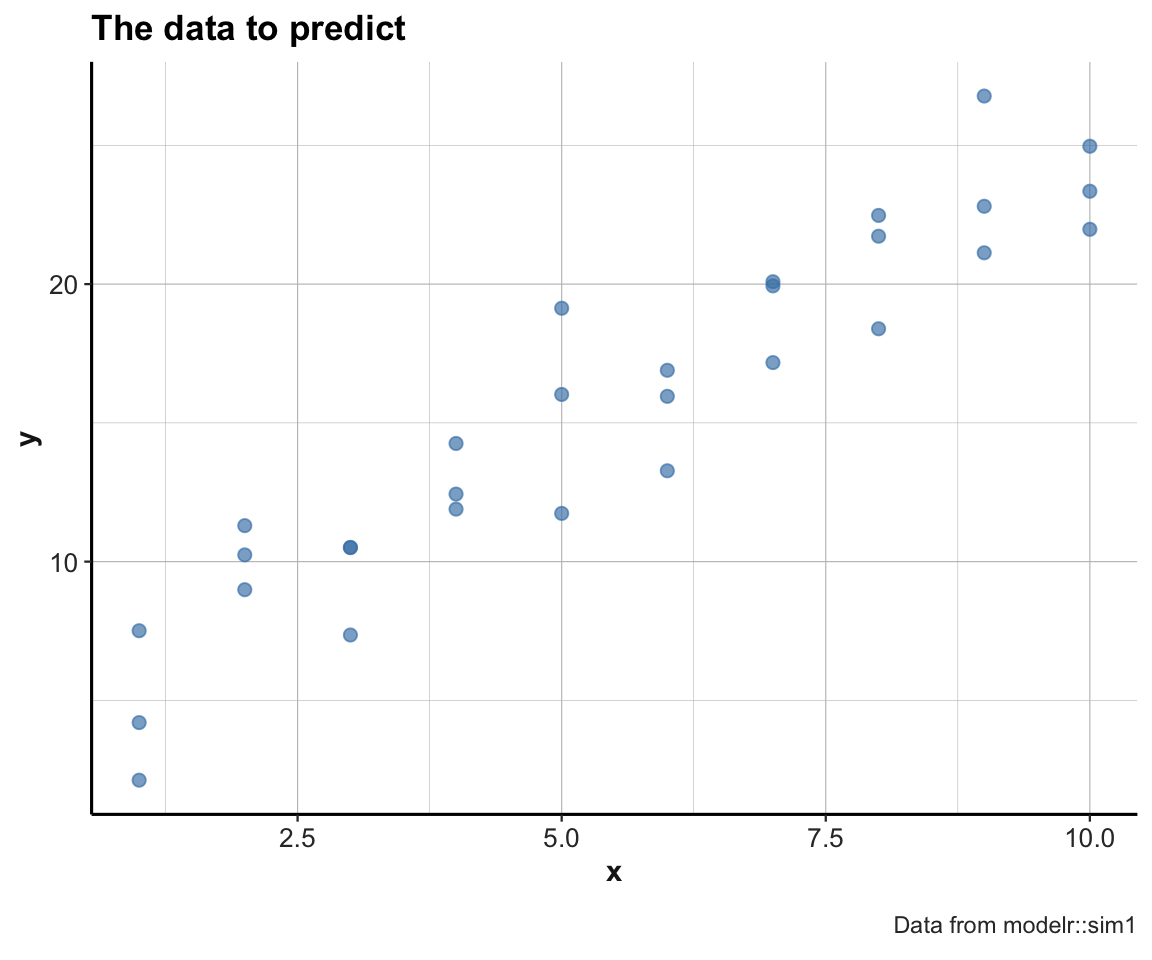
Figure 23.1: A scatterplot of the to-be-predicted data.

Random models

Generate n linear models of form y = p1 + p2 * x:

n <- 100
set.seed(246)  # for reproducible randomness. 

# Sample n random values for p1 and p2: 
models <- tibble(
  p1 = runif(n, -20, 20),
  p2 = runif(n,  -5,  5)
)

ggplot(sim1, aes(x, y)) + 
  geom_abline(aes(intercept = p1, slope = p2), data = models, alpha = 1/5) +
  geom_point(color = "steelblue", size = 2, alpha = 2/3) + 
  labs(title = "The data to predict and random linear models", caption = "Data from modelr::sim1") + 
  theme_ds4psy()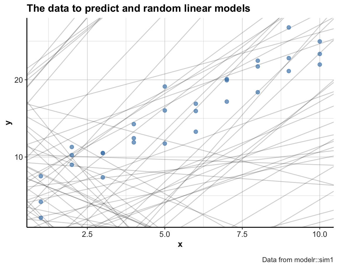

Note usage of set.seed() for reproducible randomness.

Some random linear models appear to be ok, but most of them are pretty bad (i.e., do not describe the locations and relations of the data points very well).

We can improve the quality of our models by narrowing down the range of parameters from which we sample:

set.seed(123)  # for reproducible randomness. 

# Sample n random values for p1 and p2: 
models <- tibble(
  p1 = runif(n, 0, 10),
  p2 = runif(n, 0, 5)
)

ggplot(sim1, aes(x, y)) + 
  geom_abline(aes(intercept = p1, slope = p2), data = models, alpha = 1/5) +
  geom_point(color = "steelblue", size = 2, alpha = 2/3) + 
  labs(title = "The data to predict and random linear models", caption = "Data from modelr::sim1") + 
  theme_ds4psy()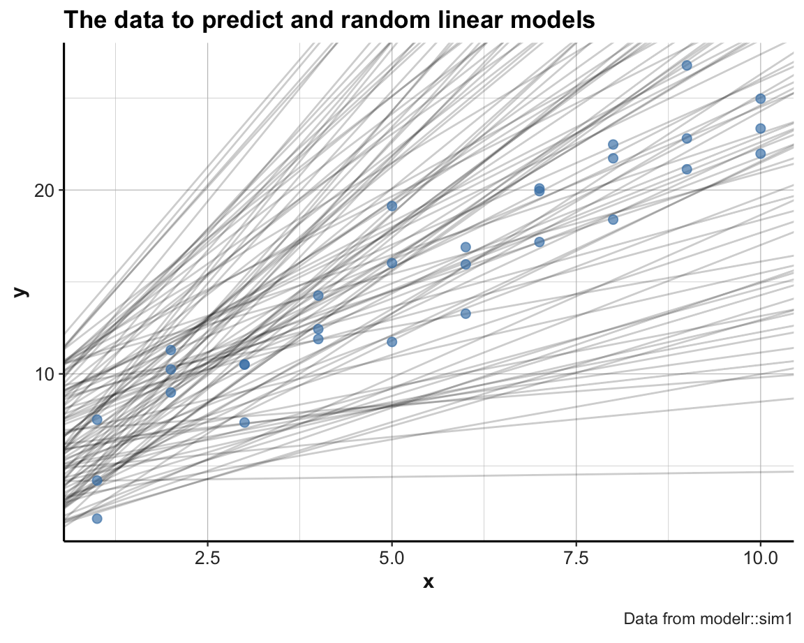

The new set of models is much better. But to determine which is the best candidate among them, we need some way of comapring them to the data in a quantitative fashion.

To measure the performance of a model, we need to quantify the distance between the model and the actual data points.

A function that computes the predictions of a model (i.e., the model’s y values for some input data data$x), given the model parameters mp:

# mp ... model parameters

# Model predictions: 
model1 <- function(model, data) {
  model[1] + model[2] * data$x 
}

# Generate predictions for various model parameters and dat:
model1(c(6, 3), dat)
#>  [1]  9  9  9 12 12 12 15 15 15 18 18 18 21 21 21 24 24 24 27 27 27 30 30 30 33
#> [26] 33 33 36 36 36
model1(c(6, 2), dat)
#>  [1]  8  8  8 10 10 10 12 12 12 14 14 14 16 16 16 18 18 18 20 20 20 22 22 22 24
#> [26] 24 24 26 26 26
model1(c(5, 3), dat)
#>  [1]  8  8  8 11 11 11 14 14 14 17 17 17 20 20 20 23 23 23 26 26 26 29 29 29 32
#> [26] 32 32 35 35 35
model1(c(5, 2), dat)
#>  [1]  7  7  7  9  9  9 11 11 11 13 13 13 15 15 15 17 17 17 19 19 19 21 21 21 23
#> [26] 23 23 25 25 25

Adding a distance function: root of the mean-squared deviation: The following function computes the difference between actual and predicted, square them, average them, and the take the square root:

distance <- function(model, data) {
  diff <- data$y - model1(model, data)
  sqrt(mean(diff ^ 2))
}

# Measure distance for models and dat: 
distance(c(6, 3), dat)
#> [1] 7.803283
distance(c(6, 2), dat)
#> [1] 2.60544
distance(c(5, 3), dat)
#> [1] 6.920964
distance(c(5, 2), dat)
#> [1] 2.190166

Alternative distance function (using 2 model parameters as two distinct arguments and only using the data of dat):

dist <- function(p1, p2) {
  distance(c(p1, p2), data = dat)
}

# Checks: 
all.equal(dist(6, 3), distance(c(6, 3), dat))
#> [1] TRUE
all.equal(dist(6, 2), distance(c(6, 2), dat))
#> [1] TRUE

We can now compute the distance of each model in models:

# using a for loop:
md <- rep(NA, nrow(models))

for (i in 1:nrow(models)){
  md[i] <- dist(models$p1[i], models$p2[i])  
}
md

# Or directly:
md_2 <- purrr::map2_dbl(models$p1, models$p2, dist)

# Verify equality:
all.equal(md, md_2)

In one step: Compute the distance of all models (generated above) and arrange by lowest distance:

models <- models %>% 
  mutate(dist = purrr::map2_dbl(p1, p2, dist)) %>%
  arrange(dist)

models  # with a column for dist
#> # A tibble: 100 × 3
#>      p1    p2  dist
#>   <dbl> <dbl> <dbl>
#> 1  4.15  2.05  2.13
#> 2  1.88  2.33  2.41
#> 3  2.32  2.20  2.43
#> 4  6.53  1.61  2.48
#> 5  5.51  2.05  2.50
#> 6  6.93  1.60  2.50
#> # … with 94 more rows
#> # ℹ Use `print(n = ...)` to see more rows

We can now select the top_n models (i.e., those with the lowest overall distance to the sim1 data) and compare them to the data:

# Plot the top models:
top_n <- 10

# subset of models to plot:
m2p <- models[1:top_n, ]  # base R solution (given that models are sorted by -dist)
m2p <- dplyr::filter(models, rank(dist) <= top_n)  # dplyr solution
# m2p

pt <- paste0("The data to predict and the top ", top_n, " random linear models")

ggplot(sim1, aes(x, y)) + 
  geom_abline(aes(intercept = p1, slope = p2, color = dist), 
              data = m2p, alpha = 4/5) +
  geom_point(color = "steelblue", size = 2, alpha = 2/3) + 
  labs(title = pt, caption = "Data from modelr::sim1") + 
       scale_color_gradient(low = "gold", high = Bordeaux) + 
  theme_ds4psy()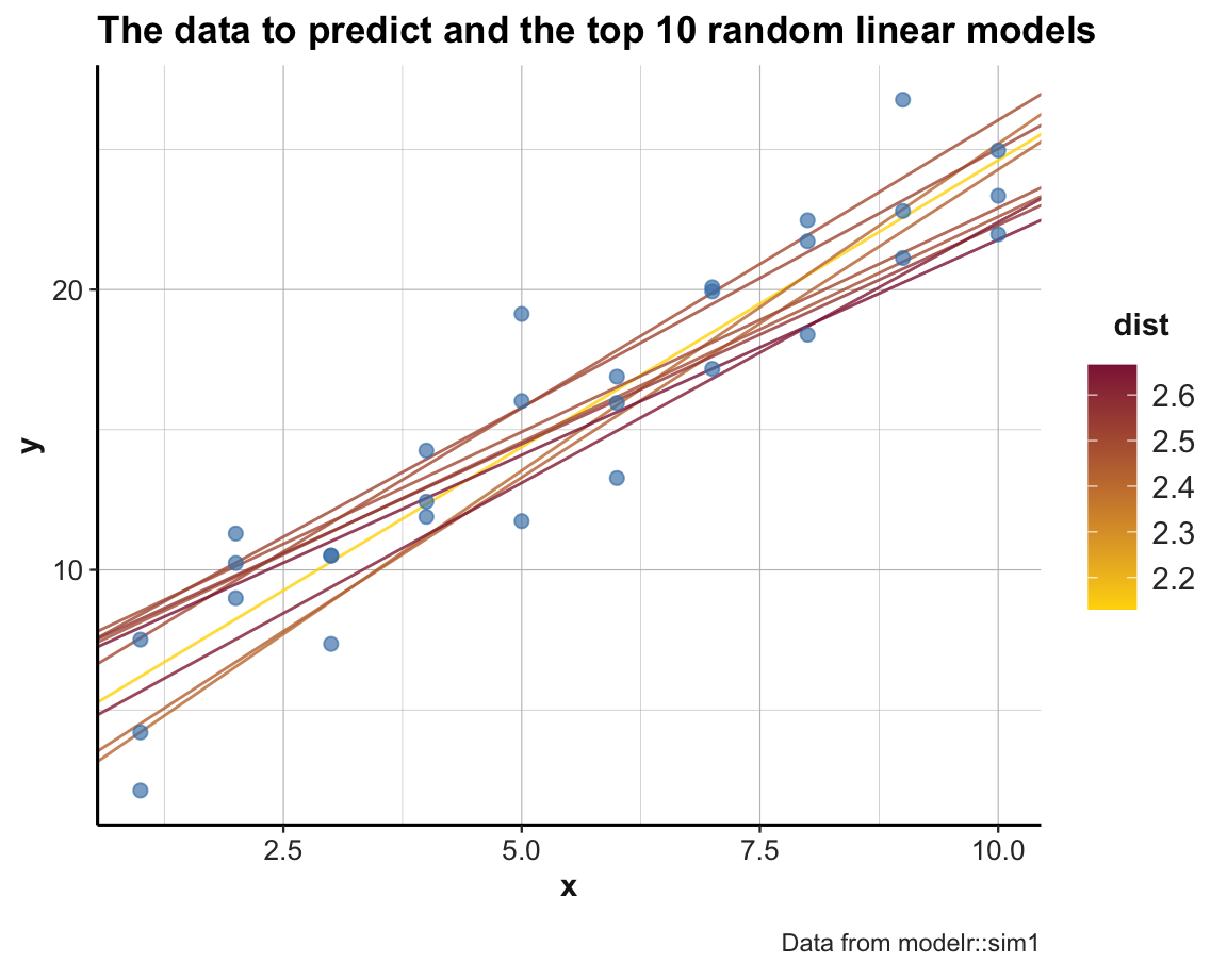

An alternative way of looking at the models is by plotting the parameter pair p1 and p2 of each model as a scatterplot. To gain an impression about a model’s performance, we can color the corresponding point by -dist (i.e., models with a lower distance value will be colored in a lighter color). Additionally, the following command first draws the subset of the top_n models in a larger size and brighter color, effectively highlighting those models in the full scatterplot:

ggplot(models, aes(p1, p2)) +
  geom_point(data = filter(models, rank(dist) <= top_n), 
             size = 4, color = Seegruen) +
  geom_point(aes(color = dist), size = 2) +
  scale_color_gradient(low = "gold", high = Bordeaux) + 
  theme_ds4psy()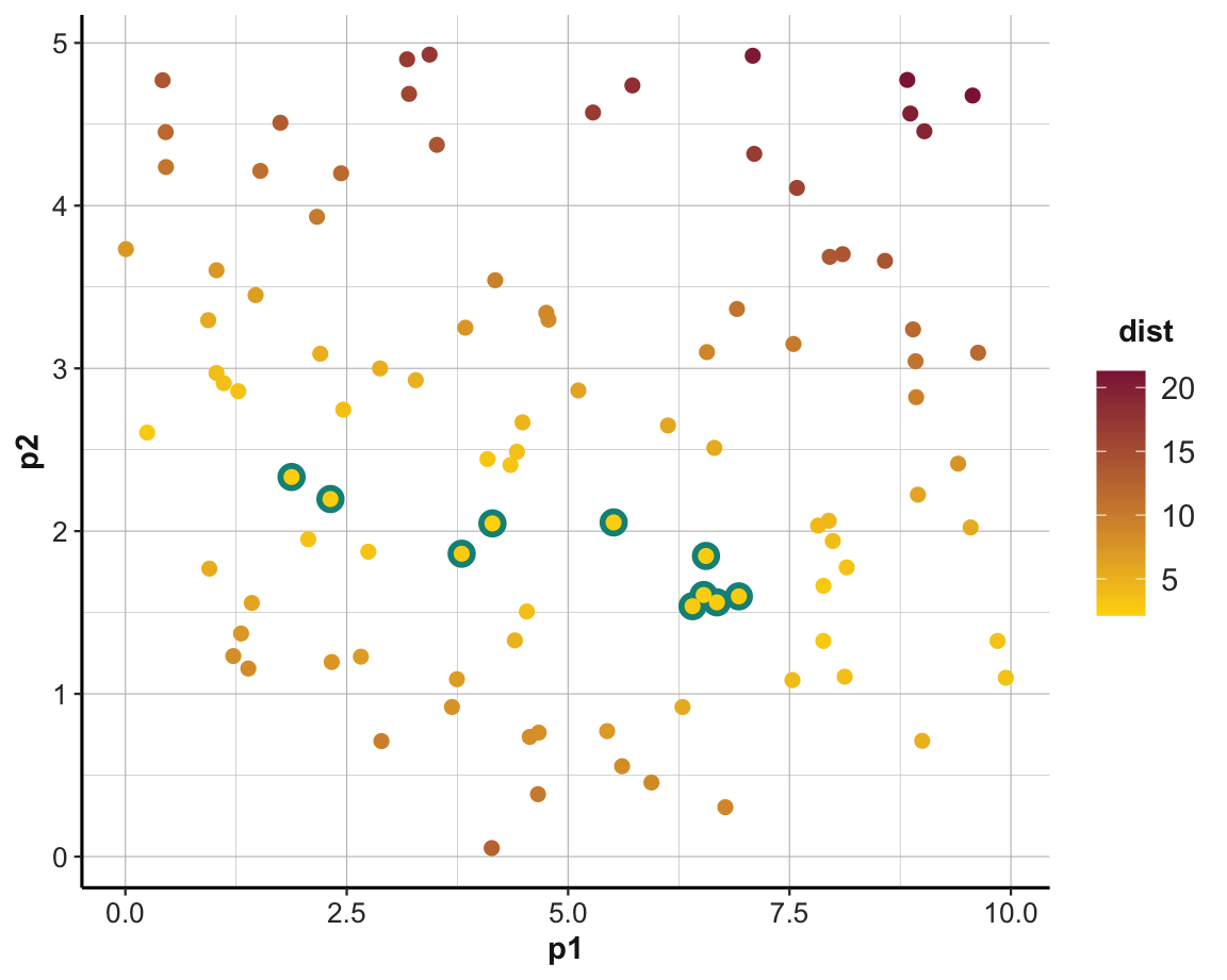

Grid search

Rather than generating model parametes randomly (within constraints), we could also generate an evenly spaced grid of points (within the same constraints).

Instead of trying lots of random models, we could be more systematic and generate an evenly spaced grid of parameters. The following creates such a grid search for $20 \times 20$ parameter pairs:

grids <- expand.grid(
  p1 = seq(0, 10, length = 20),
  p2 = seq(0,  5, length = 20)
  ) %>% 
  mutate(dist = purrr::map2_dbl(p1, p2, dist)) %>%
  arrange(dist)

# Data with grid of linear models: 
ggplot(sim1, aes(x, y)) + 
  geom_abline(aes(intercept = p1, slope = p2, color = dist), 
              data = grids, alpha = 1/5) +
  geom_point(color = "steelblue", size = 2, alpha = 2/3) + 
  labs(title = "Grid search of linear models", 
       caption = "Data from modelr::sim1") + 
       scale_color_gradient(low = "gold", high = Bordeaux) + 
  theme_ds4psy()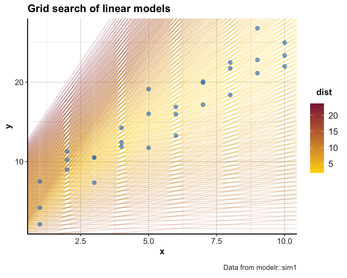


# Parameters (as scatterplot): 
ggplot(grids, aes(p1, p2)) +
  geom_point(data = filter(grids, rank(dist) <= top_n), 
             size = 4, colour = Seegruen) +
  geom_point(aes(colour = dist), size = 2) + 
  scale_color_gradient(low = "gold", high = Bordeaux) + 
  theme_ds4psy()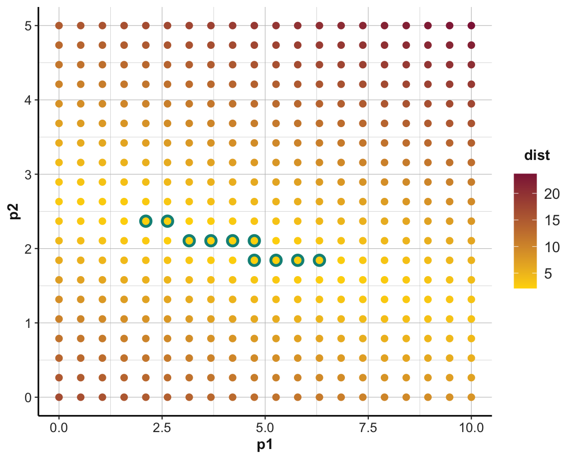

We could repeat this process for a finer grid to incrementally zoom in to the best parameters.

Minimizing distance

An important part of quantitative modeling is to find parameters that would optimize (i.e., maximize or minimize) some measure.

There are multiple ways of doing this.

If we are considering a one-dimensional range of values, the optimize() function (of the stats package) searches this range (from some lower to some upper value) for a minimum (or maximum) of the first argument of some function f:

curve(expr = (x - 1/3)^2, from = -1, to = 2, col = "deepskyblue", lwd = 2, ylab = "y")

# As a function:
fn <- function(x, a) {(x - a)^2}  # x as 1st parameter (to be optimized)

(mn <- optimize(fn, c(-1, 2), a = 1/3))
#> $minimum
#> [1] 0.3333333
#> 
#> $objective
#> [1] 0
(mx <- optimize(fn, c(-1, 2), a = 1/3, maximum = TRUE))
#> $maximum
#> [1] 1.999924
#> 
#> $objective
#> [1] 2.777525
(mx_2 <- optimize(fn, c(-1, 1), a = 1/3, maximum = TRUE)) # Note limited range
#> $maximum
#> [1] -0.999959
#> 
#> $objective
#> [1] 1.777668

# Not as lists:
# (mx <- unlist(mx))  # as named vector

points(x = mn$minimum, y = mn$objective, col = "olivedrab3", pch = 16, cex = 2)     # using mn
points(x = mx$maximum, y = mx$objective, col = "brown2", pch = 17, cex = 2)         # using mx
points(x = mx_2$maximum, y = mx_2$objective, col = "steelblue", pch = 18, cex = 2)  # using mx_2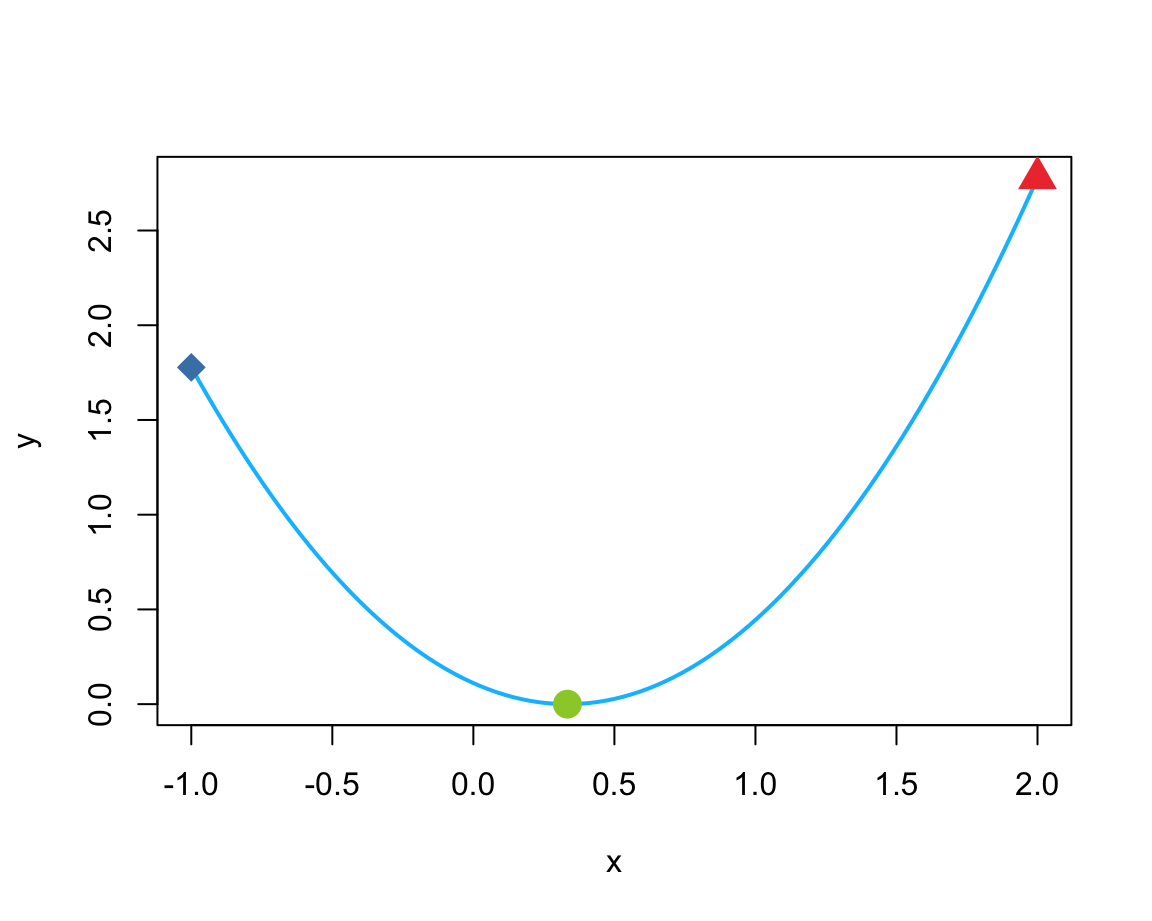

Examples based on the documentation of optimize():

# Example 2:
fn <- function(x) {x^3 * (x - 1)}
plot(fn, col = "deepskyblue", lwd = 2)

# Minimum:
(mn <- optimize(fn, lower = 0, upper = 2))
#> $minimum
#> [1] 0.7500078
#> 
#> $objective
#> [1] -0.1054687
points(x = mn$minimum, y = mn$objective, col = "olivedrab3", pch = 16, cex = 2) # using mx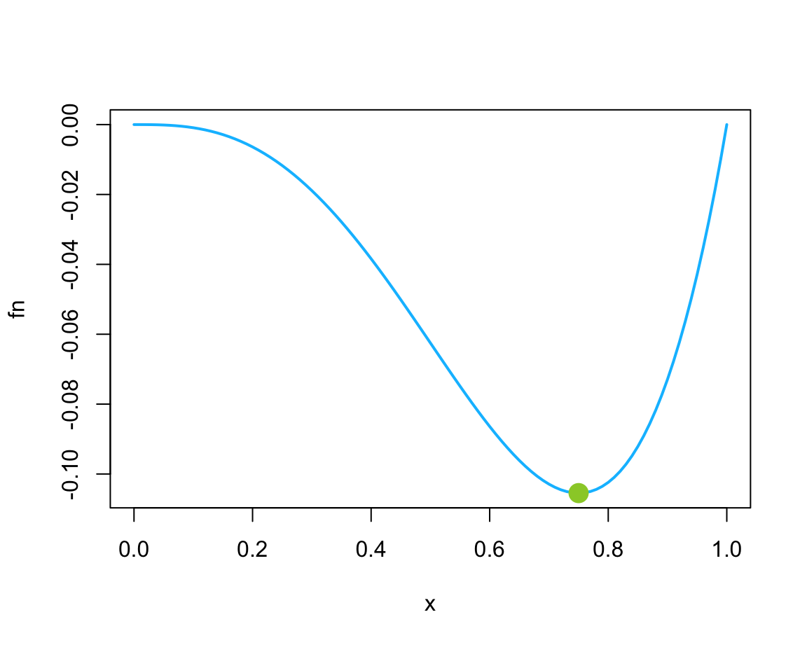


# See where a function is evaluated:
optimize(function(x) x^3 * (print(x) - 1), lower = 0, upper = 2)
#> [1] 0.763932
#> [1] 1.236068
#> [1] 0.472136
#> [1] 0.6666667
#> [1] 0.7777988
#> [1] 0.7471242
#> [1] 0.7502268
#> [1] 0.7499671
#> [1] 0.7500078
#> [1] 0.7500485
#> [1] 0.7500078
#> $minimum
#> [1] 0.7500078
#> 
#> $objective
#> [1] -0.1054687

# Warning: 
# A "wrong" solution with an unlucky interval and piecewise constant f():
f  <- function(x) ifelse(x > -1, ifelse(x < 4, exp(-1/abs(x - 1)), 10), 10)
fp <- function(x) { print(x); f(x) }

plot(f, -2,5, ylim = 0:1, col = "red")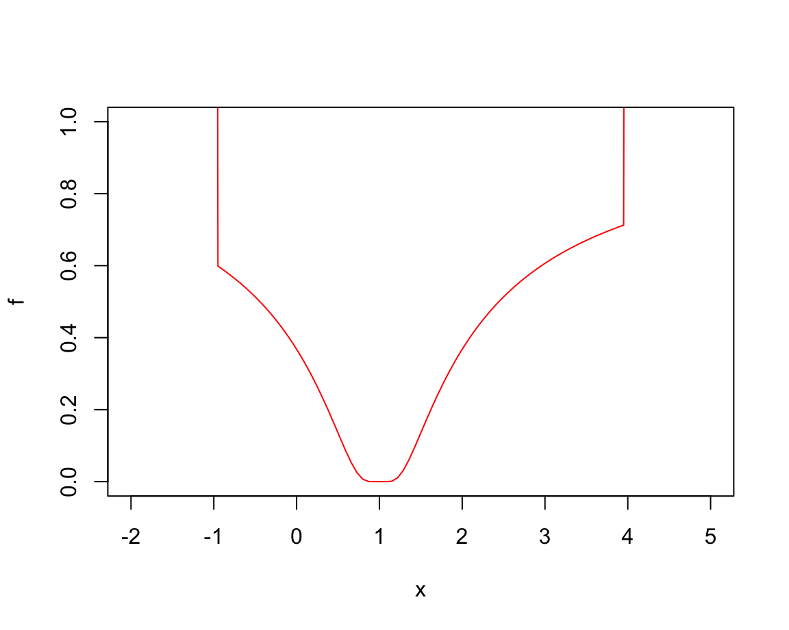

optimize(fp, c(-4, 20))   # fails to find the minimum
#> [1] 5.167184
#> [1] 10.83282
#> [1] 14.33437
#> [1] 16.49845
#> [1] 17.83592
#> [1] 18.66253
#> [1] 19.1734
#> [1] 19.48913
#> [1] 19.68427
#> [1] 19.80487
#> [1] 19.8794
#> [1] 19.92547
#> [1] 19.95393
#> [1] 19.97153
#> [1] 19.9824
#> [1] 19.98913
#> [1] 19.99328
#> [1] 19.99585
#> [1] 19.99743
#> [1] 19.99841
#> [1] 19.99902
#> [1] 19.99939
#> [1] 19.99963
#> [1] 19.99977
#> [1] 19.99986
#> [1] 19.99991
#> [1] 19.99995
#> [1] 19.99995
#> $minimum
#> [1] 19.99995
#> 
#> $objective
#> [1] 10
optimize(fp, c(-7, 20))   # finds minimum
#> [1] 3.313082
#> [1] 9.686918
#> [1] -0.6261646
#> [1] 1.244956
#> [1] 1.250965
#> [1] 0.771827
#> [1] 0.2378417
#> [1] 1.000451
#> [1] 0.9906964
#> [1] 0.9955736
#> [1] 0.9980122
#> [1] 0.9992315
#> [1] 0.9998411
#> [1] 0.9996083
#> [1] 0.9994644
#> [1] 0.9993754
#> [1] 0.9993204
#> [1] 0.9992797
#> [1] 0.9992797
#> $minimum
#> [1] 0.9992797
#> 
#> $objective
#> [1] 0
optimize(fp, c(-2, 5))   
#> [1] 0.6737621
#> [1] 2.326238
#> [1] -0.3475242
#> [1] 0.9935203
#> [1] 1.075221
#> [1] 1.034342
#> [1] 1.013931
#> [1] 1.003726
#> [1] 0.998623
#> [1] 1.001174
#> [1] 0.9998987
#> [1] 1.000538
#> [1] 1.000294
#> [1] 1.000143
#> [1] 1.00005
#> [1] 0.999992
#> [1] 0.9999513
#> [1] 0.9999513
#> $minimum
#> [1] 0.9999513
#> 
#> $objective
#> [1] 0

Here, we explore two different methods (both from the stats package that comes with R): General intuition: Given the scatterplot of our data (shown in Figure 23.1), we have a pretty good idea that we are looking for a linear model.

General-purpose optimization (using optim())
Fitting a linear model (using lm())

ad 1: Using optim() to determine the best parameter pair:

Intuition: Given a fn = distance and data, optim() will use an algorithm to find the parameter combination par that minimize the value of distance.

# sim1
best <- optim(par = c(0, 0), fn = distance, data = sim1)
best$par # vector of the 2 best parameters (i.e., minimizing fn for data)
#> [1] 4.222248 2.051204

ggplot(sim1, aes(x, y)) + 
  geom_point(color = "steelblue", size = 2, alpha = 2/3) + 
  geom_abline(intercept = best$par[1], slope = best$par[2], color = "gold") + 
  labs(title = "The best linear model to predict the data", 
       caption = "Data from modelr::sim1") + 
  theme_ds4psy()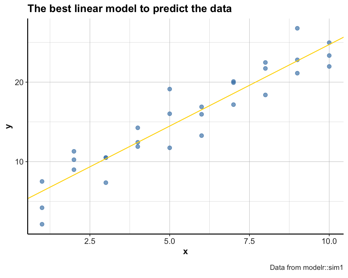

ad 2: Using lm() for fitting a linear model:

sim1_mod <- lm(y ~ x, data = sim1)
coef(sim1_mod)
#> (Intercept)           x 
#>    4.220822    2.051533

For fitting other datasets and types of functions, using glm() or nlm() may be indicated.

23.3.7 ToDo 2

Quantitative prediction/regression: Generalize and use a more meaningful dataset:

Candidate data: father.son or galton (both from the UsingR package)
analysis

See Chapter 3: Linear regression of James et al. (2021).

23.4 Qualitative prediction tasks

Qualitative prediction models address classification tasks: Assigning elements to categories.

Examples:

Screening test: Healthy tissue or signs of cancer?
Will some market or individual stock go up or down today/this month/year?
A classic task: Who survived the Titanic disaster?

Typical methods: Logistic regression, naive Bayes, Knn, and classification trees.

Strategy: Stimulate intuition by using 2x2 matrix as an analytic device. Beyond predicting category membership, we also want to evaluate the quality of the resulting prediction.

qualitatively: Predict membership to a binary category.
quantitatively: Describe result and measure success (as accuracy or some other metric).

Disclaimer

Note that this section is still unfinished.

23.4.1 Titanic data

Start with a dataset:

Binary variables

# As contingency df:
t_df <- as.data.frame(Titanic)

# with(tt, table(Survived, Sex))  # only number of cases

t2 <- t_df %>%
  group_by(Sex, Survived) %>%
  summarise(n = n(),
            freq = sum(Freq))
t2
#> # A tibble: 4 × 4
#> # Groups:   Sex [2]
#>   Sex    Survived     n  freq
#>   <fct>  <fct>    <int> <dbl>
#> 1 Male   No           8  1364
#> 2 Male   Yes          8   367
#> 3 Female No           8   126
#> 4 Female Yes          8   344

# Frame a 2x2 matrix: ------ 

# (a) Pivot summary into 2x2 matrix: 
t2 %>% 
  pivot_wider(names_from = Sex, values_from = freq) %>%
  select(-n)
#> # A tibble: 2 × 3
#>   Survived  Male Female
#>   <fct>    <dbl>  <dbl>
#> 1 No        1364    126
#> 2 Yes        367    344

# (b) From contingency df: 
xtabs(Freq ~ Survived + Sex, data = t_df)
#>         Sex
#> Survived Male Female
#>      No  1364    126
#>      Yes  367    344

# (c) From raw data cases:
t_raw <- i2ds::expand_freq_table(t_df)
table(t_raw$Survived, t_raw$Sex)
#>      
#>       Male Female
#>   No  1364    126
#>   Yes  367    344

Note the complexity of a 2x2 table interpretation, due to a difference between different measures and different perspectives that we can adopt on them. In terms of measures, we see a difference between frequency counts, proportions, and different kinds of probabilities:

Frequencies: Absolute numbers show many more males than females
Proportions of survivors by gender: Majority of females survived, majority of males died.
Probabilities can be joint, marginal, or conditional (depending on the computation of their numerator and denominator).

23.4.2 ToDo 1

Steps of the matrix lens model (see the MLM package):

Determine a pair of a predictor and a criterion variable.
Frame a 2x2 matrix:

Matrix transformations:

m_1
rowSums(m_1)
colSums(m_1)
sum(m_1)

# Get four basic values:
(abcd <- c(m_1[1, 1], m_1[1, 2], m_1[2, 1], m_1[2, 2]))

# Probabilities and marginal probabilities: 
prop.table(m_2) * 100
prop.table(m_2, margin = 1) * 100  # by rows
prop.table(m_2, margin = 2) * 100  # by cols
# ToDo: Diagnonal (margin = 3)

# Test:
chisq.test(m_1)
chisq.test(m_2)
chisq.test(m_3)

# Visualization:
mosaicplot(t(m_2), color = c("skyblue1", "grey75"))
mosaicplot(t(m_3), color = c("skyblue1", "grey75"))

Focusing: Compute various metrics
When predictor variable is continuous (and criterion is binary): Determine an optimal cut-off point to maximize some criterion.

23.4.3 Trees

Goal: Illustrate cases of binary prediction by the FFTrees package (Phillips et al., 2017).

library(FFTrees)
library(tidyverse)

t_df <- FFTrees::titanic
t_tb <- as_tibble(t_df)
t_tb

## variables as factors:
# t_tb$survived = factor(t_tb$survived, levels = c(1, 0))
# t_tb$sex = factor(t_tb$sex, levels = c("female", "male"))

t_tb

t4 <- t_tb %>%
  group_by(class, age, sex, survived) %>%
  count()
t4

t3 <- t_tb %>%
  group_by(sex, survived) %>%
  count()
t3

xtabs(cbind(survived, sex) ~ ., data = t_tb)

# Pivot into 2x2 matrix: 
t3 %>% 
  pivot_wider(names_from = sex, values_from = n)

Resources

Statistical methods for tackling classification tasks:

See Chapter 4: Classification of James et al. (2021).

Note existing resources for cross-tabulations:

Consider using the tab_xtab() and plot_xtab() functions from the sjPlot package.
See examples at Chapter 8: Cross-Tabulation of R you Ready for R? (by Wade Roberts)

23.5 Conclusion

23.5.1 Summary

Prediction is the hallmark of useful knowledge: Explanation without prediction remains useless speculation.

Technically, prediction requires an association between variables, but correlation does not yet imply causation (or mechanistic explanation).

A predictive model should answer three key questions:

What is being predicted? What type of predictive task is being performed?
How is predictive success evaluated?
What is the baseline performance and the performance of alternative benchmarks?

Actually, asking these three questions are useful for any kind of agent modeling or measuring performance in general. (See Neth et al., 2016, for applications in assessments of human rationality.)

23.5.2 Beware of biases

A final caveat:

A story: Inspecting WW-II bomber planes after their missions: Assume that

90% of planes show bullet hits on wings;
10% of planes show bullet hits on tanks.

Where should we add more reinforcements?

An instance of survivorship bias.

More generally, we may be susceptible to biases due to the availability of data. Thus, when training and evaluating algorithms, we must always ask ourselves where the data is coming from.

23.5.3 Resources

Pointers to sources of inspirations and ideas:

Books, chapters, and packages

The distinction between regression tasks and classification tasks in this chapter is based on James et al. (2021):

Chapter 3: Linear Regression (James et al., 2021)
Chapter 4: Classification (James et al., 2021)

Other chapters and/or books:

Chapter 10: Predictive modeling of Modern Data Science with R (Baumer et al., 2021)
Tidy Modeling with R aims to extend the tidyverse to data modeling. The tidymodels framework provides a suite of R packages that applies the tidyverse design philosophy to modeling.

Prediction in R

The statistical analysis of predictive models often implies linear regression (LR) models. The following links provide helpful introductions and analyses:

The SOGA-R) project provides nice explanations and examples (in geodata contexts):

Multiple LR analysis: A simple example explains the statistics of predictive modeling in R and provides an example of multiple linear regression analysis (using the trees data)
Multiple LR analysis: An advanced example

Reference: Hartmann, K., Krois, J., Rudolph, A. (2023): Statistics and Geodata Analysis using R (SOGA-R). Department of Earth Sciences, Freie Universitaet Berlin.

Articles and blogs

The Learning Machines blog (by Holger K. von Jouanne-Diedrich) provides many posts on essential aspects of prediction. For instance:
- The post ZeroR: The simplest possible classifier shows why high accuracy can be misleading.
- The post Learning data science: Modelling basics introduces basic notions of quantitative models in R (including model fitting and overfitting).

23.6 Exercises

23.6.1 Predicting game outcomes in sports

A simple model for predicting possible outcomes of soccer games needs to assign probabilities to possible outcomes. For instance, when playing a soccer game, the outcome is determined by the number of goals scored by each team. If we can capture the probabilities of scoring goals, we can predict the probability of specific outcomes.

Study the following posts at the Learning Machines blog:

Tasks to address:

Find some relevant data (ideally of an entire season) and tidy it. What are key variables that allow predicting game performance?
Creating a model: Build a model that predicts the outcomes of games.
Validation: Predict some outcomes in your data, and compare them to the actual outcomes.
Out of sample prediction: Predict the outcomes for the next season and comapre them to the actual outcomes.
Transfer to other tasks and domains:
- What would change when we wanted to predict the outcome in another type of sport (e.g., boxing, basketball)?
- What would change when we wanted to predict the outcome of political elections?

22 Social situations

24 R pour l’art

23 Prediction

Preparation

Preflections

23.1 Introduction

23.2 Essentials of prediction

23.2.1 Explaining vs. predicting

23.2.2 Examples

23.2.3 Types of tasks

23.2.4 Evaluating predictive success

23.2.5 Baseline performance and other benchmarks

23.3 Quantitative prediction tasks

Disclaimer

23.3.1 Introduction

23.3.2 A basic model

23.3.3 Linear models

Model accuracy

Correlation

Linear regression

Standardizing model variables

Key elements of a model

Fitting vs. predicting

Evaluating the accuracy of model predictions

23.3.4 Comparing models

23.3.5 Multiple predictors

23.3.5.1 Practice

23.3.6 Notes on regression modeling

Introduction

Random models

Grid search

Minimizing distance

23.3.7 ToDo 2

23.4 Qualitative prediction tasks

Disclaimer

23.4.1 Titanic data

23.4.2 ToDo 1

23.4.3 Trees

Resources

23.5 Conclusion

23.5.1 Summary

23.5.2 Beware of biases

23.5.3 Resources

Books, chapters, and packages

Prediction in R

Articles and blogs

Related R packages

23.6 Exercises

23.6.1 Predicting game outcomes in sports