19 Modeling
This chapter on Modeling introduces the new book part on Applications. Before we will learn how to create basic and more complex simulations in R, we need to reflect on the nature, goals, and criteria of scientific models.

Figure 19.1: German cover of the iconic song by Kraftwerk from 1978. (Image from Wikipedia/Kling Klang.)
Models do not only perform on fashion runways, but also on stages and computers. Figure 19.1 shows the cover of the Die Mensch-Maschine (i.e., the man-machine), an iconic album by the German electronic music pioneers Kraftwerk (see this YouTube video for a studio performance from 1980). In 1981, the song was released on the studio album Computer World and as the B-side of a single of the song entitled Computerliebe (i.e., computer love, see Figure 19.2):

Figure 19.2: UK single cover. (Image by EMI/Kling Klang.)
In the following, we will mostly consider computer models, but should not lose sight of the larger implications of modeling for both science and society.
Preparation
Note that this chapter is still unfinished.
Recommended readings for this chapter include:
- Chapter 2: Statistical learning of the book An introduction to statistical learning with applications in R (ISLR) by James et al. (2021).
Related resources include:
- Materials at StatLearning.com (including book PDF, data, code, figures, and slides)
- R package ISLR2
- A summary script of the chapter is available here
Note that the term statistical learning refers to a variety of models and can be used as a synonym for modeling.
Preflections

Before reading on, please take a moment to reflect on the following questions:
What is a model? What is modeling?
What are the goals of models and modeling?
Who and what determines whether a model is good or bad?
19.1 Essentials of modeling
If ‘data is the new oil’, then models are the new pipelines
— and they are also refineries.Erica Thompson (2022, p. 12)
The scientific revolution (see Wikipedia) — often linked to the Renaissance of the 15th and 16th century AD and the age of reason and enlightenment — is intimately related to the use of scientific models. Although astronomers, mathematicians, and scholars from other disciplines have always been using theoretical models, the emergence of science based on the collection of data and systematic experimentation led to a proliferation of all kinds of models. One of the earliest and most influential protagonists of this revolution was the Italian polymath Leonardo da Vinci (1452–1519, see Wikipedia) whose journals, drawings, and sketches merge an obsession with detail with an intense curiosity for bold inventions. Figure 19.3 shows his drawing of the Vitruvian Man (see Wikipedia), which anchors the study of anatomical proportions in both art and science:
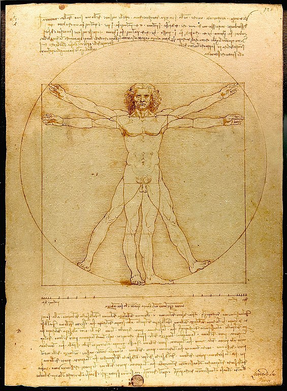
Figure 19.3: The Vitruvian Man by Leonardo da Vinci, around 1490. (Photograph by Luc Viatour/Lucnix.be.)
This chapter aims to clarify some key concepts (models vs. simulations vs. statistics) and provides some historical background and examples. For the rest of the book, we need to reflect on the goals of modeling (see Section 19.1.4) and the criteria by which models can and should be evaluated (see Section 19.1.5).
19.1.1 Terminology
What is a model and what is modeling?
We will adopt the following definitions:
A model is an abstract and formal structure that provides a simplified description of a phenomenon and aims to capture its essential elements.
By contrast, modeling is the activity and methodology of creating, running, and evaluating such models.
Noteworthy elements of these definitions include:
-
A mathematical model is an abstract structure that captures structure, patterns, and processes in the data (Luce, 1995).
- “abstract” implies simplification
- “structure” implies regularity
Thus, a miniature replica would be a poor “model”, as it would be as complex as the original.
A description or structure does not per se yield hypotheses, predictions, or data. To gain any of these, models must be interpreted, instantiated, run, and evaluated. This is the purpose of modeling.
As models are typically represented in some formalism (e.g., diagrams or mathematical formulas), they can be expressed and executed in computer code.
Models are often discussed in the same contexts as scientific theories and paradigms. The term paradigm literally denotes a model or pattern, that serves as an example or typical instance of something. The role of paradigms in the history of science was popularized by T. S. Kuhn (1962), who defines a scientific paradigm as “universally recognized scientific achievements that, for a time, provide model problems and solutions for a community of practitioners” (p. 10). Thus, a scientific paradigm usually denotes the larger context within which more specific models are being developed. A paradigm defines the type and scope of problems that scientists are willing or able to address in their everyday routines of constructing and evaluating models.
We will mostly use the term model to denote specific instantiations of scientific theories and hypotheses. If science was organized in neat set/subset relations, a paradigm would contain many theories, and theories would contain many models. However, reality is more messy and involves blurred boundaries, overlapping categories, and outliers that do not fit into these categories.
19.1.2 Model types vs. levels
There are many types and typologies of scientific models (i.e., ignoring those used to advertise and fit products in design and fashion). Many characterizations of models emphasize particular mathematical constructs (e.g., linear vs. non-linear models), disciplines (e.g., statistical vs. machine learning models), or technologies (e.g., computer models, R models).
Basics: Medium/How the model is formulated?
- verbal vs. formal models (abstract, parameterized)
Examples: Verbal theories that postulate three instances (e.g., super-ego, ego, and id) or two systems (fast vs. slow) can easily accommodate a wide variety of phenomena. Unless they are specified further, they are so vague and flexible that it remains unclear how much of their narrative appeal translate into concrete predictions.
A nice example for a verbal claim that seems innocuous, but may actually be vacuous is provided by Hintzman (1991) (p. 41): A familiar claim from a sociobiology textbook is the following:
While adultery rates for men and women may be equalizing,
men still have more partners than women do, and they are
more likely to have one-night stands(Leahey & Harris, 1985, see Google books for context and full quote).
Hintzman (1991) criticizes verbal theories and issues the challenge of constructing an actual model. According to him, such statements may sound plausible, but risk making “a mathematically impossible claim” (p. 41). Building a model would force the authors to explicate what they mean by “more partners” — and there are interpretations that would not be “mathematically impossible” (see Exercise 19.3.4).
- Distinction within formal models: mathematical vs. computer models
Corresponding remarks:
- Model types: We can distinguish between different types of models: (1) formal models (abstract, using mathematical formalisms) and (2) simulations (concrete, instantiations). However, the boundaries are blurred, as any thing, construct, or symbol (e.g., a number) can be represented in a variety of ways.
Typology by Lewandowsky & Farrell (2011): Three increasingly deep types of models are models that
- describe the data;
- describe the process;
- explain the process.
An alternative to categorizing models into types consists in asking: At which level of analysis do models attempt to explain a phenomenon?
An analytically useful one stems from neuroscientist David Marr (1945–1980, see Wikipedia), who studied the physiology of the visual system. According to Marr (1982), we can study cognition at three complementary but distinct levels of analysis:
The computational level: What task does the system address? What problems does it solve and why does it face and solve them?
The algorithmic/representational level: How does the system do what it does? Specifically, what representations does it use and what processes does it employ to create and manipulate them?
The implementational/physical level: How are the system and its processes physically realised? What neural circuits, structures, and processes implement the system?
Importantly, we can construct models at each level. Thus, different types of models will serve different goals and generate or explain different types of data. [See Lewandowsky & Farrell (2011), for an alternative typology.)
- Historically, the idea of using a model or simulation for predicting outcomes is not new (see e.g., Craik, 1943; Gentner & Stevens, 1983; Johnson-Laird, 1983). But creating models has become much easier with the ubiquity of computers and tools that allow us to create and evaluate models.
19.1.3 Examples
Models are being used in many realms of life and all scientific disciplines. Some examples of models include:
- astronomy: geocentric vs. heliocentric models of the universe or solar system
- anthropology: mythology as narrative accounts of history
- medicine: soul in heart vs. brain
- finance: fundamental vs. technical analysis of stock markets
- psychology: mind as a clock vs. as a computer
- climate research: models of atmospheric layers, and global warming
It is instructive to consider the transition between scientific theories and models in more detail. One of the most prominent models in the history of science concerns the position and role of our planet in the solar system.
The Ptolemaic model
In the 2nd century AD, the Hellenistic mathematician, geographer and astronomer Claudius Ptolemaeus (see Wikipedia) standardized a geocentric model of our universe. In this model, Earth is viewed as a sphere in the center of the cosmos. Each planet is moved by a system of two spheres, known as deferent and epicycle. Figure 19.4 illustrates these basic elements of Ptolemaic astronomy. A planet is rotating on an epicycle which is itself rotating around a deferent inside a crystalline sphere. In Figure 19.4, the system’s center is marked by the X, and our earth is slightly shifted off-center. Opposite the earth is its equant point, which is the center around which the planetary deferent is actually believed to rotate.
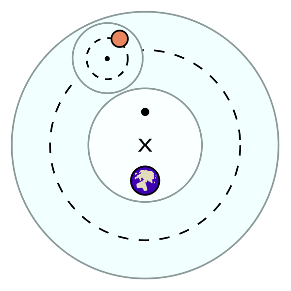
Figure 19.4: Key elements of the Ptolemaic model of a geocentric universe. (Image from Wikimedia commons, not drawn to scale.)
By all reasonable accounts, the Ptolemaic model was widely successful: It predicted different kinds of celestial motions with high accuracy and was used and taught by generations of astronomers. After more than a millenium, the model was challenged in the 16th century by the heliocentric account of Nicolaus Copernicus’ (see Wikipedia). However, as the Copernican system erroneously assumed circular orbits of the planets around the sun, it was no more accurate than Ptolemy’s system. Despite its merits in simplicity, the heliocentric account faced strong opposition by contemporary natural philosophy and religious doctrine (see the trials of Giordano Bruno and Galileo Galilei).
The consensus on the Ptolemaic model only faded in the 17th century, when empirical observations by Johannes Kepler (see Wikipedia) and his heliocentric model with elliptical planetary orbits provided a superior account.36
Thus, “being right” is rarely the reason for adopting a new model — and requires a verdict that is only available in hindsight. Instead, replacing a dominating scientific model can take a long time and often faces considerable resistance by established authorities. (See T. S. Kuhn (1962) and Lakatos & Feyerabend (1999) for the philosophical background.)
Models in psychology
Models of mental processes are particularly tricky. Is the occurrence of a global pandemic best explained by some invisible virus or by the will of God? When we feel stressed by professional or private challenges, should we look into our personality traits, some lack of skills, or for repressed childhood memories? Our cultural history provides a rich compendium of anecdotal, mythological, religious, and scientific models that offer competing explanations for any turn of events or whim of fate.
An important realization: It is easy to “explain” phenomena in verbal terms. For instance, equipped with some “systems”, like Freud’s three instances (super-ego, ego, id) or the more modern so-called “dual-process” theories (i.e., the interaction of a fast/intuitive and a slow/deliberate system) pretty much everything and its opposite can easily be explained. The problem with this is that explanations that always work for everything are vacuous, as they are impossible to falsify. Thus, a good model is not one that explains everything, but a model that is specific enough to fail and can be replaced by a better model.
Models force us to be explicit about assumptions, parameters, and processes. By checking whether our intuitions about some hypothetical system matches what actually arises from its implementation, models act as insurance policies against speculative leaps. Thus, models provide several benefits that are absent from narrative accounts. They
make scientific thinking more reproducible,
allow us to avoid common mistakes that may bias our intuitive reasoning, and
facilitate the communication about psychological capacities and processes
See Farrell & Lewandowsky (2010) for a more detailed version of this argument.
19.1.4 Goals
What is the goal of modeling?
Most people intuitively anwer that a model must be an accurate copy of the phenomenon it represents. But whereas a certain degree of accuracy may be necessary feature of a good model, it cannot be a sufficient one. For instance, the most accurate model of a brain would be the brain itself (or an exact replica of it). However, unless we can construct, examine, and understand the model, having access to the most accurate model is completely intransparent and useless.
By contrast, a mathematical formula that predicts a physical phenomenon is very different from the phenomenon itself. For instance, the decrease of atmospheric temperature~\(T\) with increasing altitude~\(z\) can be described and predicted by the so-called Lapse rate: \(\Gamma = -\frac{dT}{dz}\). However, nothing about this model is particularly warm/cold or high/low.
Thus, the main criterion for evaluating a model is not truth or accuracy, but whether the model is useful. And as usefulness is a functional term, it always depends on the goals and purposes for which the model is designed.
The goal of modeling is succinctly summarized in the following statement (Wickham & Grolemund, 2017):
The goal of a model is not to uncover truth,
but to discover a simple approximation that is still useful.Wickham & Grolemund (2017), Ch. 23: Model basics
Wickham & Grolemund (2017) further relate this to the famous aphorism that “all models are wrong”:
Since all models are wrong the scientist must be alert to what is importantly wrong.
It is inappropriate to be concerned about mice when there are tigers abroad.
The corresponding Wikipedia entry cites the following section (from G. E. Box, 1979):
Now it would be very remarkable if any system existing in the real world could be exactly represented by any simple model. However, cunningly chosen parsimonious models often do provide remarkably useful approximations.
For example, the law PV = RT relating pressure P, volume V and temperature T of an “ideal” gas via a constant R is not exactly true for any real gas, but it frequently provides a useful approximation and furthermore its structure is informative since it springs from a physical view of the behavior of gas molecules.
For such a model there is no need to ask the question “Is the model true?”. If “truth” is to be the “whole truth” the answer must be “No”. The only question of interest is “Is the model illuminating and useful?”.
Thus, rather than aiming to approximate truth, models aim to be useful constructs that contain intentional simplifications.
The basic distinction between explanation and prediction does not exhaust potential goals of modeling. For instance, the REDCAPE acronym by Page (2018) distinguishes seven different uses of models:
- Reason: Identify conditions and deduce logical implications.
- Explain: Provide testable explanations for phenomena.
- Design: Choose features of institutions, policies, or rules.
- Communicate: Relate knowledge and understanding to others.
- Act: Guide policy choices and strategic actions.
- Predict: Predicting future or unknown (categorical or numerical) phenomena
- Explore: Investigate hypothetical cases and possibilities.
Interestingly, meeting some of these criteria is difficult, but not sufficient to guarantee a “good” model. For instance, so-called black box models may exhibit impressive capacities (e.g., see the “stochastic parrots” by Bender et al., 2021), yet lack transparency and merely mimic the underlying mechanisms. Similarly, a model’s ability to explain phenomena is usually an attractive property, but may be unmasked as a plausible “just-so story” when it provides inaccurate predictions, fails to provide actionable insights, or we find an even better model (see Thompson, 2022, p. 42f.).
Rather than discussing the benefits and pitfalls of a particular model, a helpful approach consists in viewing models as metaphors or alternative perspectives (Thompson, 2022). How useful a model will be depends less on its intrinsic properties than on the circumstances in which it is created and its use and purpose in some historical and social context.
One side-effect of this perspective is that we can abandon our quest for a single unifying model and embrace model diversity. For instance, Page (2018) advocates such a many-model approach: Rather than searching for the “right” model, we can gain insights by viewing our problem through a multiplicity of lenses.
Summarizing possible goals of modeling requires that we spell out different aspects of “usefulness”:
- scope: address or categorize phenomena
- accuracy: describing data
- insight into mechanisms: explaining data
- predictive power
- parsimony: abstraction and simplicity
- aesthetics: elegance and beauty
Some of the later goals (like simplicity or elegance) may only matter when the accuracy, explainability, and predictive power of models are comparable. Also, these goals can be turned into criteria for evaluating models, but depend on the context and purpose for which they are being used.
19.1.5 Evaluating models
What determines the merits or success of a model?
- A model’s quality always depends on its purpose: What is considered “essential” depends on our purposes. For deciding which clothes to pack for a vacation, having a weather model that shows the range of average temperature values for each month may be good enough. However, for predicting the temperature for hiking trip over the next two days, such a coarse model may be inadequate.
Note that both instances of a temperature model would still be judged by the same metric (e.g., a comparison between predicted and measured temperature, where we would ask for smaller deviations for a near-term prediction than for a long-term prediction). However, we often would want to use more than one criterion (e.g., not just temperature, but also expected amounts of sunshine or precipitation). In fact, most real-world models will typically be evaluated on multiple critera.
The range of criteria for evaluating models mirror the aspects of “usefulness” (from above):
- scope: which phenomena are addressed or categorized
- accuracy: fit to or distance from data
- insight into mechanisms: explaining data
- predictive power: ability to predict phenomena of interest
- parsimony: abstraction and simplicity
- aesthetics: elegance and beauty
Statistical models
Formal models in many natural sciences often appear in the form of statistical models. Although this book is not on statistics, any interest in formal models needs to briefly discuss three elementary dichotomies in statistics:
Sample vs. population: When formulating hypotheses or theories, we typically address populations of entities. Howerver, our data rarely contains observations of entire population. Instead, we collect data from samples and analyze them in order to infer characteristics of the underlying population.
Data as “information given” (experienced or observed) vs. model as an abstract description of data: A (verbal/mathematical/statistical) model describes (given) data, but can also be used to generate new data.
Explanation vs. prediction (or “inference”): Correspondingly, data can be used to explain or verify a model, or to predict new/unobserved data (aka. “inference”).
Overall, the activities of data collection and modeling are not iterative and mutually exclusive, but rather describe a cyclical process.
Data in models
Data serves two very distinct functions in models:
- generate hypotheses
- evaluate and test predictions
Importantly, data often is a finite resource. Thus, it is very important to use the available data in a sensible and smart fashion.
Typically: Dividing data into two main parts that are being used for fitting vs. for prediction.
See Chapter 5 Spending our data of Tidy Modeling with R for ways of sampling and splitting data.
19.1.6 Summary
Note that lists of goals of modeling (as in Section 19.1.4) could also be used to explicate the goals of science in general. Thus, the methodology of modeling lies at the very core of conducting science.
Overall, models are essential tools for thinking about the interplay of theory and data. As with any method or tool, models can be used wisely or unwisely. Figuring out which models are useful and how to use models wisely is a key purpose of science.
19.2 Conclusion
Overall, models are indispensable tools for thinking and for making sense of data. They explicate theoretical assumptions, identify essential parts and processes, allow to reason and evaluate predictions, provide existence proofs for hypothesized mechanisms, inform actions and policies, and enable scientists and other stakeholders to understand and communicate results.
Despite these benefits, we end on a cautionary note: The fact that models are indispensable does not imply that we should blindly trust their results, of course. Like any method or tool, models can be used wisely or unwisely. Any model-based result is only as good as the assumptions and data that went into its creation. Even small deviations from seemingly arbitrary premises or slight perturbations in parameters can result in vastly different results. Importantly, these crucial dependencies are often obscured by an overall impression of formal rigor and mathematical precision. A careful examination of models should always take into account their variability and uncertainty. If, however, their results are taken at face value, a blind reliance on models can be dangerous and border on religious idolatry. For instance, Pilkey & Pilkey-Jarvis (2007) argue that many of the quantitative models that politicians and administrators use to guide environmental policies are seriously flawed. When models are based on unrealistic or false assumptions, they can be used to support unwise or even harmful policies.
19.2.1 Summary
Here is a brief summary of key terms and insights:
Models are (formal or informal) descriptions of phenomena. They are tools or methodological vehicles that help us grasp the world.
Creating and evaluating models is the activity of modeling.
Explanatory models allow us to design, reason, and explore scenarios.
Thus, models can help to explicate assumptions, parameters, and processes, that otherwise remain implicit and vague.Explanation is cheap. Successful models should also be good at predicting empirical phenomena. Predictions can be categorical or numerical.
Models have multiple goals: Models are never “true”, but rather aim to be useful. An important use of models lies in making ideas and processes more communicable to and verifyable by others. Successful models can also guide actions and policies.
19.2.2 Resources

Some pointers to resources for inspirations and ideas on models, modeling, and simulations:
Books on modeling in R
There are many good books on models and modeling. As the tradition of data modeling is much older than that of R or current R packages, students should not be tempted to read only the most recent textbooks, but rather stick to established classics.
Modeling in R and the tidyverse is an area with a very long tradition (under the name of statistics and machine learning) and many active developments. Although we often tend to favor recent tools and resources, many of them are partial and unfinished. Hence, we recommend starting with the basics and acquiring some sound background knowledge that allows evaluating the most recent developments.
Solid recommendations include:
-
An introduction to statistical learning (ISLR) book by James et al. (2021).
Related resources include:
- Materials at StatLearning.com (including book PDF, data, code, figures, and slides)
- R package ISLR2
- Data school videos on statistical learning
-
Applied predictive modeling by M. Kuhn & Johnson (2013).
Related resources include:- Materials at AppliedPredictiveModeling.com
When aiming for models of psychological processes, the books by Lewandowsky & Farrell (2011) and Farrell & Lewandowsky (2018) provide solid introcuctions with many examples in R.
-
Modern Data Science with R by Baumer et al. (2021) provides a simpler and more general introduction:
- Available online at https://mdsr-book.github.io/mdsr2e/
Valuable contributions with some rough or unfinished parts:
Statistical Inference via Data Science (by Chester Ismay and Albert Y. Kim) provides a hands-on approach to modeling in R and the tidyverse.
Chapters 22 to 25 of the r4ds book (Wickham & Grolemund, 2017).
The R packages at tidymodels.org provide a collection of tools for modeling and machine learning in accordance with tidyverse principles. The emerging book Tidy Modeling with R (by Max Kuhn and Julia Silge) aims to show how to use them.
Blogs and online sites
All models are right, most are useless: Andrew Gelman’s StatModeling blog, (2012-03-04)
The Learning Machines blog (by Holger K. von Jouanne-Diedrich) discusses engaging topics of data science and provides numerous inspirations for a wide range of data science projects. The post on Learning Data Science: Modelling Basics is a good place to start (although it discusses quantitative models that we only consider in Chapter 23 on Prediction).
Disentangling data science provides additional inspirations
Visualization
- Hannah Yan Han medium page and associated GitHub project
Machine Learning
The term data science is often used as an alternative name for statistical learning or machine learning:
100 days of ML code: in Python, but great infographics
Miscellaneous
More models by Leonardo da Vinci:
- Scientific drawings and inventions (on Wikipedia |
- on YouTube: Leonardo: Anatomist, by Nature Video, 2012)
More Kraftwerk soundtracks for computer modeling:
Man-machine (on Wikipedia | on YouTube: full album, 1978 | remasterd version, 2009)
Computer love (on Wikipedia | on YouTube: 7-min version | extended 1-hour version)
The model (on Wikipedia | on YouTube: in English, remastered version | string version by the Balanescu Quartet, 2011)
19.3 Exercises

19.3.1 Model revolutions
Sketch an instance of a scientific revolution that resulted in a fundamental new model of some discipline or domain. (Candidates include cosmological, biological, chemical, medical or physical phenomena.)
What was the established model that was replaced by a new one?
Was the transition from old to new model smooth or bumpy? How long did it take?
What were the benefits and costs of the new model? Which new predictions were enabled by it?
Hints: This exercise uses the term model in a loose way, not distinguishing it from scientific theories or paradigms. A good starting point for corresponding searches is the classic text by T. S. Kuhn (1962).
Solution
ad 1.: There are many candidates for fundamental shifts in scientific perspectives. Examples include the shift from the cardiocentric hypothesis (see Wikipedia) to the cephalocentric perspective (see Wikipedia).
ad 2.: Most shifts are quite bumpy and messy, as several conflicting perspectives can co-exist for some time, before one gains a decisive advantage over the other(s). Depending on the domain and models, this may take anything from years to centuries.
ad 3.: This depends on the nature and purpose of the models considered. For instance, conducting heart or brain surgery requires a different neurophysiological understanding than speculating about the seat of her soul.
19.3.2 Miniature model
In May 2021, the German news site Spiegel Online reported on the efforts of Reinhold Dukat, who re-constructed a miniature version of the Würzburg cathedral (St. Kilian’s dome, see Wikipedia) out of approx. 2.5 million Lego pieces (see Figure 19.5):
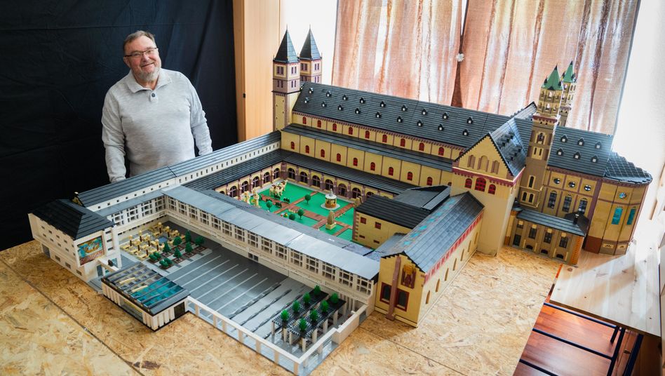
Figure 19.5: A proud architectural modeler. (Image by Nicolas Armer/dpa at SPON on 2021-05-05.)
This is undoubtedly an impressive achievement. We will seize the occasion to reflect further on the nature of scientific models.
Does creating this model make Mr. Dukat a scientist?
Which characteristics of a scientific model does his model have? Where does it fall short?
In a similar vein: Discuss how drawing a map (e.g., of a city or region) may constitute a model.
Would a satellite image of the area be a better model than a hand-drawn sketch?
Solution
ad 1.: Scientists use many models, but creating a model does not necessarily make someone a scientist. For instance, children, architects, or engineers create various models, but these are typically built for non-scientific purposes. By contrast, scientists create models for answering scientific questions (i.e., their models are means towards achieving scientific ends).
As it is possible to use a miniature replica of a building for answering scientific questions (e.g., regarding its aesthetic properties, or safety issues in emergency situations), we cannot exclude that Mr. Dukat is a scientist. However, any such judgment should be based on the questions addressed by the model, rather than on the model itself.ad 2.: Building a smaller and simpler replica of a complex phenomenon can be useful features of scientific models. Additionally, re-creating a model out of different pieces and materials imply some level of abstraction.
However, looking like an original or recreating a building in as many detail as possible are not scientific goals per se. Accuracy has many different facets and is only one of many criteria for evaluating scientific models.ad 3.: A map is a miniature representation that may or may not be a good model of the city or landscape it represents. Its utility depends primarily on the questions addressed by it. The main purpose of a map consists in facilitating orientation and navigation tasks. For many tasks, an abstract and simple model can be as useful as a more detailed and naturalistic model.
19.3.3 An almost perfect model
Measure or create some data by rolling a fair dice 100 times and recording its outcomes in data:
Create a simple model with perfect fit and perfect explanationory power:
model <- dataNote that model could be implemented as an artificial neural network or as a universal Turing machine made out of toilet paper rolls. Here, we chose to implement model in the circuits of a computer that stores information in binary form on some silicon-based device and allows explaining and predicting data as the elements of a linear vector.
Let’s evaluate the performance of our model:
# Perfect explanation:
data[13]  # individual data point
#> [1] 3
model[13]
#> [1] 3

sum(model == data)/length(data)  # overall
#> [1] 1
This shows that our model successfully captures the structure in our data.
In fact, any point in data is perfectly predicted and explained by the corresponding entry in model.
Thus, the scatterplot of Figure 19.6 shows that model provides a perfect model of data:
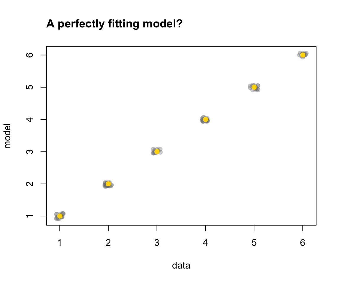
Figure 19.6: A scatterplot showing a perfect fit between data and model (showing 100 points jittered around true value).
What’s wrong with the model fit shown in Figure 19.6?
Argue why
model— despite its impressive elegance and perfect performance — may not be a such good model.Someone proposes an alternative model that goes by the name of probability theory. It assumes that any event in
datais independent of all other events and occurs with a probability of \(\frac{1}{6}\). However, this model is more complicated and its fit to the observed data is only about 16.7%. Could this still be a better model thanmodel? (Argue why or why not.)
Solution
ad 1.: As
modelis a copy ofdata, it is not surprising that it perfectly describes every point. Unfortunately, it also provides no benefit overdata. For instance, it falls short in terms of simplicity: Rather than providing an abstract description of the data, it is exactly as complex as the data. Additionally, it perfectly explains past data, but is unlikely to provide a benefit (beyond a random baseline model) in predicting new data in the future.ad 2.: The alternative model of probability theory is both more abstract and more flexible than
model. Despite providing a less accurate description of existingdata, this model is equally successful in describing new data. Its key benefit is that it provides a general account that — provided that its assumptions hold — can be applied to many similar problems (e.g., coin flips, lotteries, etc.).
19.3.4 A vague verbal model
As a warning against the potential pitfalls of merely verbal theories, Hintzman (1991) (p. 41) cited the following claim from a sociobiology textbook:
While adultery rates for men and women may be equalizing,
men still have more partners than women do, and they are
more likely to have one-night stands(Leahey & Harris, 1985, see Google books for context and full quote).
According to Hintzman (1991), this statement may sound plausible, but is actually “mathematically impossible” (p. 41). Although we agree with the general point (that verbal theories are often vague and overly permissive), his challenge requires a narrow interpretation of “more partners”.
Create a model (or a sketch) that depicts an equal number of individuals from two (or more arbitrary) genders that entertain heterosexual relationships with the other gender in some imbalanced fashion. More specifically,
In which sense is it “mathematically impossible” that men have more partners than women?
In which other sense is it possible?
Note: The quoted statement only mentioned two genders (M and W) and heterosexual relations. This does not deny more diverse situations, but they are not the focus of this exercise.
Solution
Figure 19.7 shows a hypothetical constellation with possible relations between two genders (M and F):
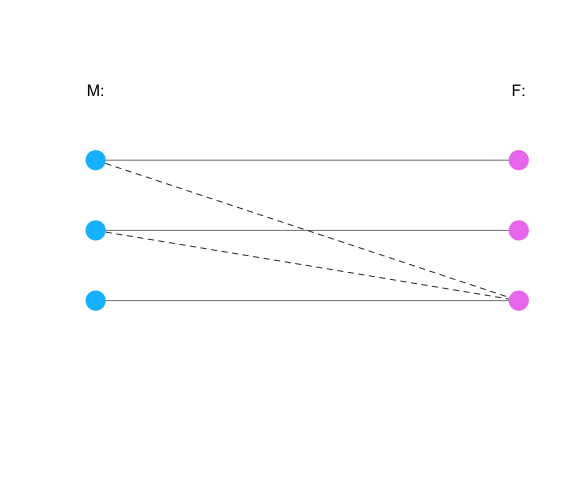
Figure 19.7: An abstract illustration of possible relations between two genders (M and F). (Dashed and solid lines depict different types of heterosexual relationships.)
Assuming that the dashed and solid lines depict different types of relationships, we can see that
ad 1.: It is impossible that the average number of relationships of M is higher than the average number of F. This is true for any number or type of heterosexual relationship, as it would always involve both genders.
ad 2.: However, it is possible that more Ms (or a higher proportion of Ms) have more than one heterosexual relationship than (the proportion of) Fs. In the situation shown here, 2 out of 3 Ms have more than one relationship, whereas only 1 out of 3 Fs has multiple relationships.
Note that this example adopts the binary and hetero-sexual perspective that corresponds to the above quote from a sociobiology textbook. This says nothing about the nature of the depicted individuals and relationships (shown as solid or dashed lines), nor does it endorse or deny the existence of other genders or relationship types. Irrespective of the popularity and value of such debates, our point here is a formal one.
Thus, the original statement must have implied a difference in the proportions among individuals of the two genders, rather than a difference in the absolute or average number of relationships. (Note that showing a possible model does not imply its actual truth, of course. Otherwise, the mere fact that the moon could be made of cheese would make this true as well…)
19.3.5 Modeling samples of famous people
In this exercise, we will conduct and compare some summary statistics on population vs. sample data. As we rarely have the data of an entire population, we will use a very large dataset and pretend that it represents a population. A reasonable approximation is the following:
Browse the Pantheon site to get an impression of its data contents and variables.
Go to https://pantheon.world/data/datasets to download a recent version of the Pantheon dataset (A. Z. Yu et al., 2016).
Load the data into R and establish its dimensions.
Solution
library(tidyverse)
library(ds4psy)
library(unikn)

# Load data:
fm <- readr::read_csv("data-raw/person_2020_update.csv")
dim(fm)
#> [1] 88937 34- Conduct an EDA on the data (as the “population” of famous people).
Solution
- Missing vs. complete cases:
## (1) Quick summaries:
# summary(fm)
# tibble::glimpse(fm)
# skimr::skim(fm)

# (1b) Missing vs. complete cases:
sum(is.na(fm))           # missing values?
#> [1] 574735
sum(complete.cases(fm))  # complete cases?
#> [1] 14

# (1c) Fix capitalization:
fm$occupation <- capitalize(tolower(fm$occupation))- Alive vs. dead:
# (2) Alive vs. dead?
fm_t2 <- fm %>%
  group_by(alive) %>%
  summarise(n = n(),
            pc = n/nrow(fm)*100)
fm_t2
#> # A tibble: 2 × 3
#>   alive     n    pc
#>   <lgl> <int> <dbl>
#> 1 FALSE 41366  46.5
#> 2 TRUE  47571  53.5

ggplot(fm_t2, aes(x = alive, fill = alive, y = pc)) +
  geom_bar(stat = "identity") +
  geom_text(aes(label = round(pc, 1), vjust = 2)) +
  labs(title = "Famous people dead vs. alive",
       x = "Alive?", y = "Percentage", fill = "Alive:") +
  scale_fill_manual(values = c("grey60", "palegreen3")) +
  theme_ds4psy()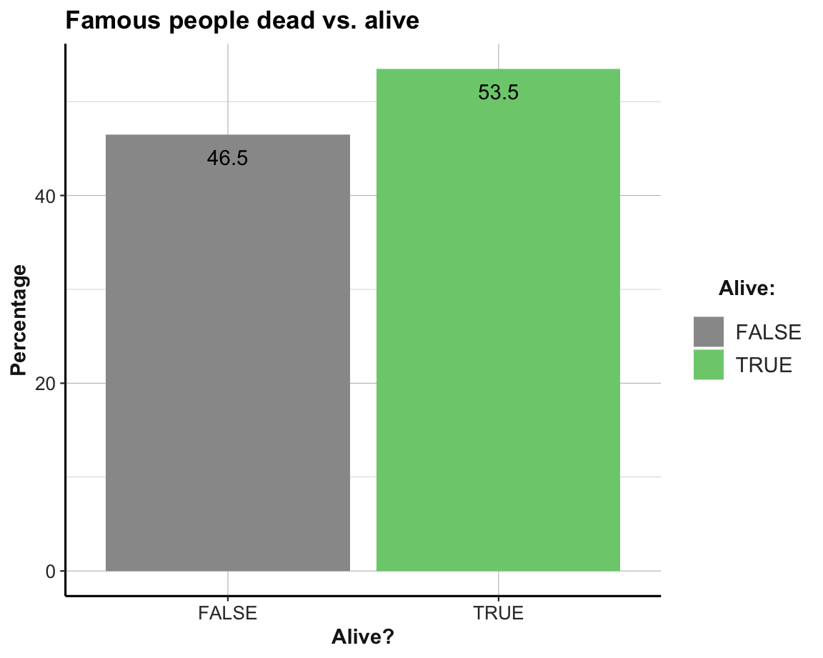
- Gender distribution:
# (3) Gender distribution:
fm_t3 <- fm %>%
  group_by(gender) %>%
  summarise(n = n(),
            pc = n/nrow(fm)*100)
fm_t3
#> # A tibble: 3 × 3
#>   gender     n      pc
#>   <chr>  <int>   <dbl>
#> 1 F      19993 22.5
#> 2 M      68928 77.5
#> 3 <NA>      16  0.0180

ggplot(fm_t3, aes(x = gender, fill = gender, y = pc)) +
  geom_bar(stat = "identity") +
  geom_text(aes(label = round(pc, 1), vjust = 2)) +
  labs(title = "Gender share", x = "Gender", y = "Percentage", fill = "Gender:") +
  scale_fill_manual(values = c("rosybrown2", "deepskyblue1", "firebrick")) +
  theme_ds4psy()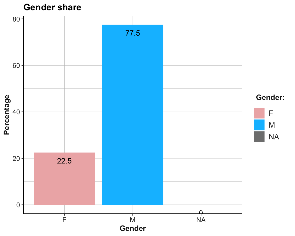
- Occupations:
# (4) Occupations:
fm_t4 <- fm %>%
  group_by(occupation) %>%
  summarise(n = n(),
            pc = n/nrow(fm)*100) %>%
  arrange(desc(n))
fm_t4
#> # A tibble: 101 × 3
#>   occupation        n    pc
#>   <chr>         <int> <dbl>
#> 1 Soccer player 16923 19.0
#> 2 Politician    15640 17.6
#> 3 Actor         10017 11.3
#> 4 Writer         5777  6.50
#> 5 Singer         3544  3.98
#> 6 Athlete        3061  3.44
#> # … with 95 more rows
#> # ℹ Use `print(n = ...)` to see more rows

ggplot(fm) +
  geom_bar(aes(x = reorder(occupation, -table(occupation)[occupation]),
               y = ..count../sum(..count..)), fill = "deepskyblue3") +
  geom_hline(yintercept = c(.05, .10, .15, .20), linetype = 3) +
  labs(title = "Occupations of famous people",
       x = "Occupation", y = "Percentage") +
  coord_flip() +
  theme_minimal() +
  theme(axis.text.y = element_text(size = rel(0.75)))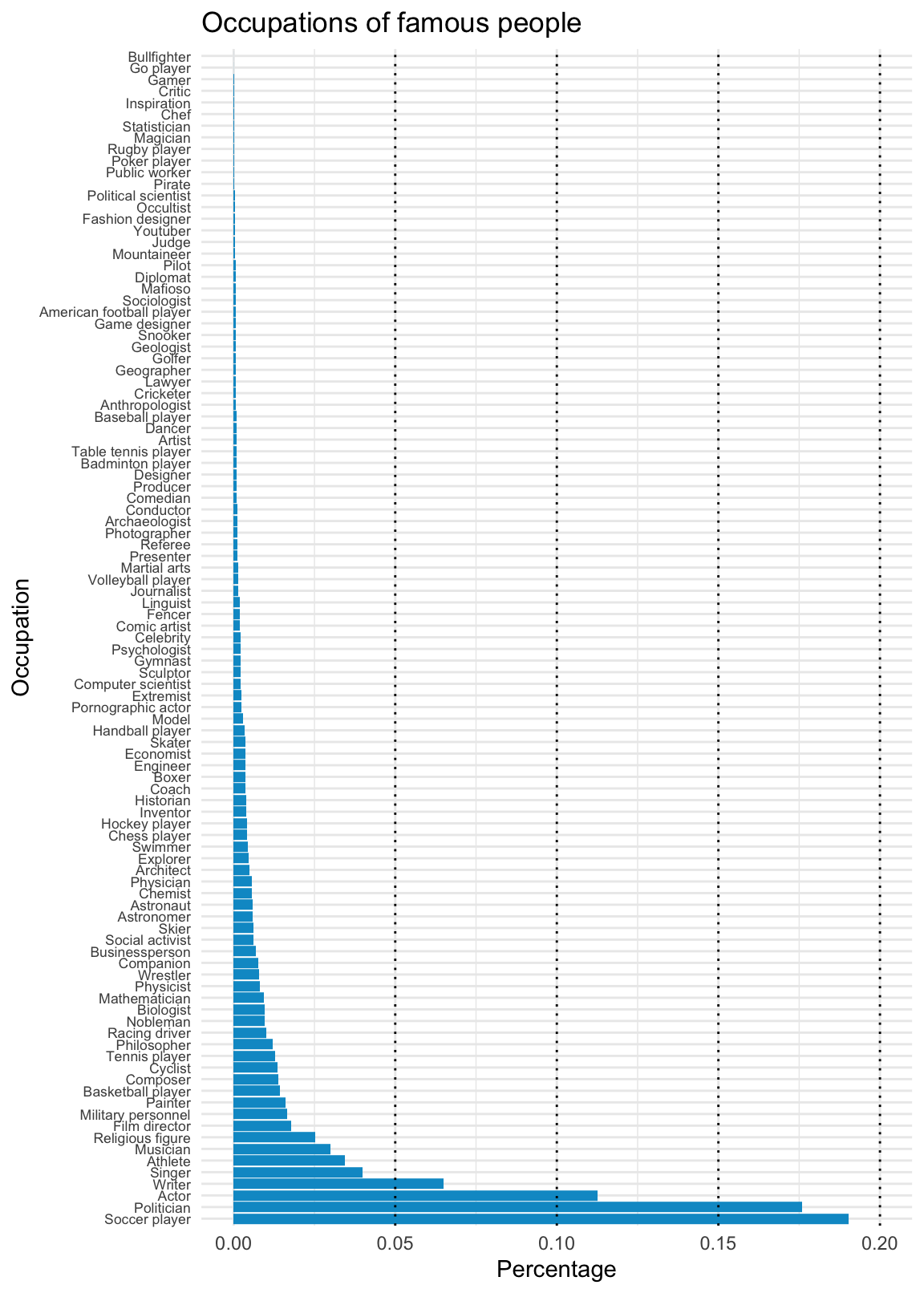
- Occupation by alive vs. dead:
# (4b) Occupation x Alive:
ggplot(fm) +
  geom_bar(aes(x = reorder(occupation, -alive, mean),
               y = ..count../sum(..count..), fill = alive), pos = "fill") +
  geom_hline(yintercept = c(.25, .50, .75), linetype = c(3, 2, 3)) +
  labs(title = "Occupations of famous people alive vs. dead",
       x = "Occupation", y = "Percentage", fill = "Alive:") +
  scale_fill_manual(values = c("grey60", "palegreen3")) +
  coord_flip() +
  theme_minimal() +
  theme(axis.text.y = element_text(size = rel(0.75)))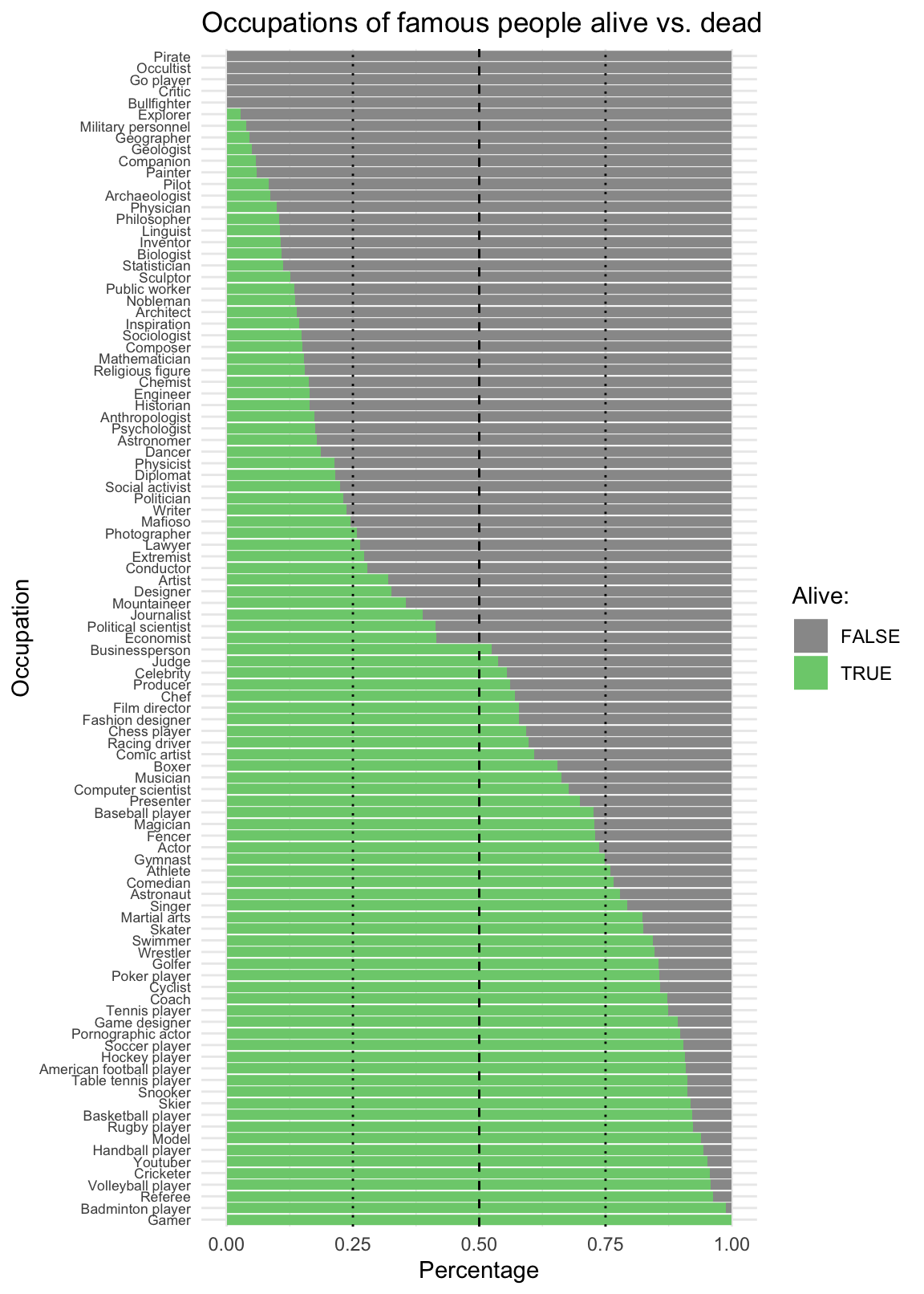
- Occupation by gender:
# (4c) Occupation x Gender:
fm_f <- fm %>%
  filter(!is.na(gender)) %>%
  mutate(female = ifelse(gender == "F", 1, 0))
# table(fm_f$female)

ggplot(fm_f) +
  geom_bar(aes(x = reorder(occupation, female, mean),
               y = ..count../sum(..count..), fill = gender), pos = "fill") +
  geom_hline(yintercept = c(.25, .50, .75), linetype = c(3, 2, 3)) +
  labs(title = "Occupations of famous people by gender",
       x = "Occupation", y = "Percentage", fill = "Gender:") +
  scale_fill_manual(values = c("rosybrown2", "deepskyblue1")) +
  coord_flip() +
  theme_minimal() +
  theme(axis.text.y = element_text(size = rel(0.75)))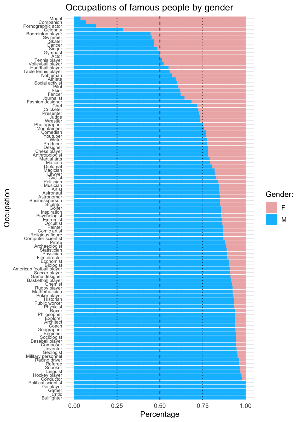
From this overview, it is pretty obvious that the data contains substantial biases. This is not surprising: Being famous is largely a matter of definition — and the inclusion criteria in any such collection will inevitably vary as a function of time and the prevailing societal norms.
- Draw a sub-sample (e.g., only people from some country, only people still alive, vs. a random subset) and repeat your analyses from 4. How does your sample compare to the population data? Which one is more representative?
Solution
It is clear from our general EDA that selecting cases based on gender and occupations will yield highly biased samples.
- We illustrate this by selecting the subset of females in professions in which females are a majority:
fm_fem_occu <- fm %>%
filter(!is.na(gender)) %>%
group_by(occupation) %>%
mutate(n_occupation = n()) %>%
ungroup() %>%
group_by(gender, occupation) %>%
mutate(n_gender_occupation = n(),
p_gender_occupation = n_gender_occupation/n_occupation) %>%
select(name, occupation, n_occupation:p_gender_occupation) %>%
filter(p_gender_occupation > .5, gender == "F") %>%
arrange(p_gender_occupation)
fm_fem_occu
#> # A tibble: 3,599 × 6
#> # Groups: gender, occupation [10]
#> gender name occupation n_occupation n_gender_occupation p_gender_…¹
#> <chr> <chr> <chr> <int> <int> <dbl>
#> 1 F Nadia Comăneci Gymnast 183 92 0.503
#> 2 F Larisa Latynina Gymnast 183 92 0.503
#> 3 F Olga Korbut Gymnast 183 92 0.503
#> 4 F Olga Tass Gymnast 183 92 0.503
#> 5 F Věra Čáslavská Gymnast 183 92 0.503
#> 6 F Ágnes Keleti Gymnast 183 92 0.503
#> # … with 3,593 more rows, and abbreviated variable name ¹p_gender_occupation
#> # ℹ Use `print(n = ...)` to see more rows
nrow(fm_fem_occu)
#> [1] 3599
# Numbers:
fm_fem_occu %>%
group_by(occupation) %>%
summarise(n = n(),
pc = n/nrow(fm_fem_occu) * 100,
pc_female = mean(p_gender_occupation) * 100) %>%
arrange(desc(pc))
#> # A tibble: 10 × 4
#> occupation n pc pc_female
#> <chr> <int> <dbl> <dbl>
#> 1 Singer 1839 51.1 51.9
#> 2 Companion 636 17.7 93.1
#> 3 Model 240 6.67 96.4
#> 4 Swimmer 215 5.97 54.8
#> 5 Pornographic actor 194 5.39 87.4
#> 6 Skater 168 4.67 53.3
#> # … with 4 more rows
#> # ℹ Use `print(n = ...)` to see more rows
# Relative frequency:
ggplot(fm_fem_occu) +
geom_bar(aes(x = reorder(occupation, -table(occupation)[occupation]),
y = ..count../sum(..count..)), fill = "deepskyblue3") +
geom_hline(yintercept = c(.05, .10, .15, .20), linetype = 3) +
labs(title = "Famous females in occupations with mostly females",
x = "Occupation", y = "Percentage") +
coord_flip() +
theme_minimal() +
theme(axis.text.y = element_text(size = rel(0.75)))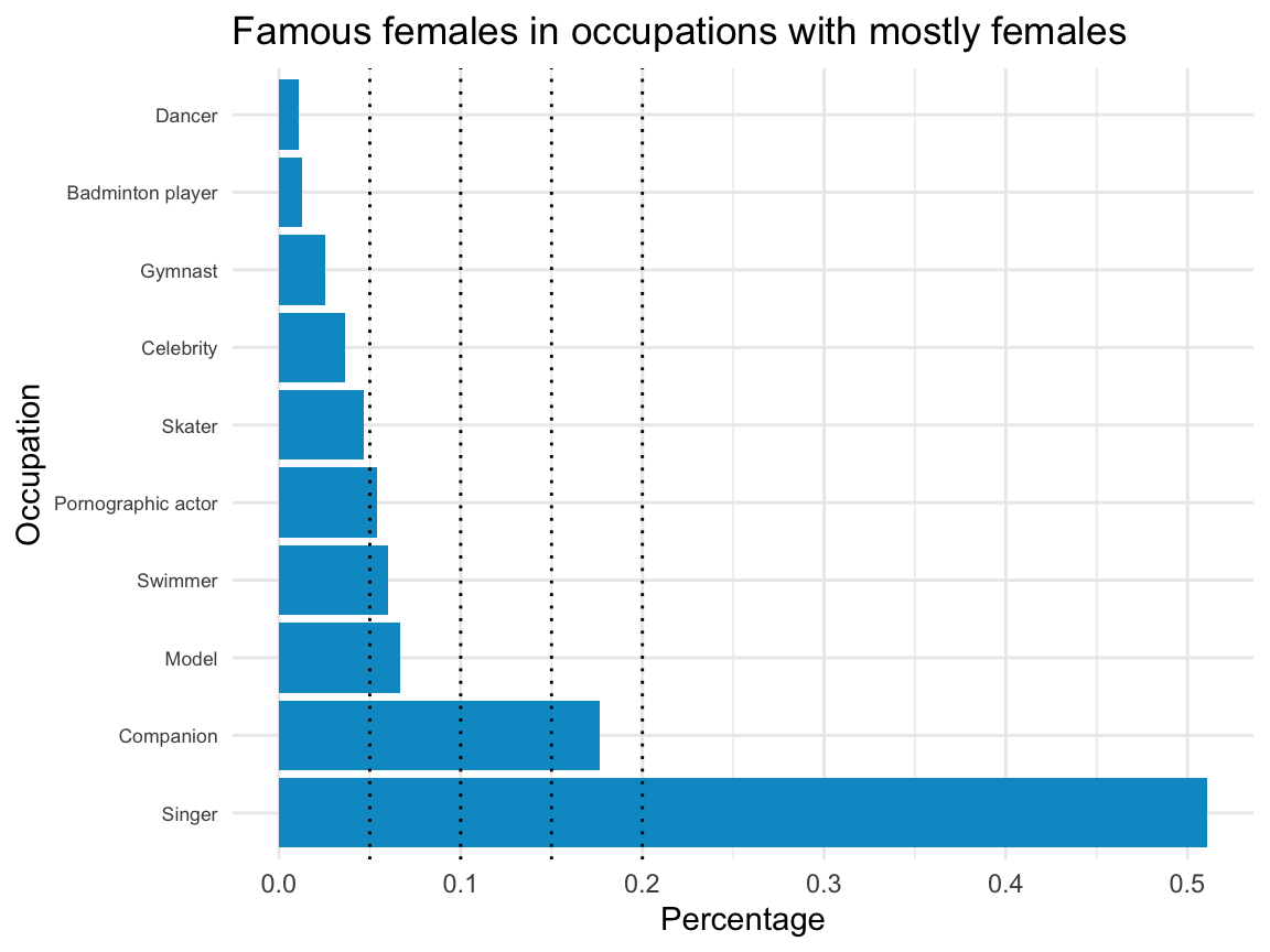
In this particular sample (still containing 3599 individuals), more than 75% are singers, companions, or models. This narrow range of professions with predominantly female individuals is due to a combination of two factors:
The inclusion criteria of the Pantheon data;
Our sample criteria (here: females in professions with a majority of females).
Interestingly, each step may seem quite innocuous in itself, but their combination paints a very biased and bleak impression of female celebrity. We can hope that this one-sided image will become more balanced and diverse in future iterations of similar data.
Overall, neither our sample nor the original data can be considered to be “representative” of humanity, of course. Instead, both samples provide insights in the mechanisms and potential consequences of collecting such data. Thus, our highly biased sample reveals that the Pantheon data also reflects deep-rooted biases in our cultural history. Such biases are common in any large dataset and illustrate why it is indispensable to always explicate our criteria for considering and including cases.
For some historical context, note that Kepler’s astronomical work was interrupted by the need to defend his mother, Katharina Kepler, against a charge of practicing witchcraft.↩︎