5 Functions

Writing our own functions will change our way of interacting with R. To put this step into perspective, consider the old proverb:

Give people a fish, and you feed them for a day.
Teach people to fish, and you feed them for a lifetime.

When applied to R, this means that the existing R functions and packages may serve us well for quite a while, but eventually we will want to write your own functions. As most analogies, likening learning R to fishing to feed oneself has its limitations. As we discussed in Chapter 1, R provides a toolbox and comes with many tools to address a variety of tasks on different levels of abstraction (see Sections 1.2.4 and 1.2.5). Thus, learning to use R’s rich arsenal of functions is quite an accomplishment and enables us to address a wide variety of tasks. And just as we usually feel no need to design a new hammer whenever we want to hit a nail, there is nothing wrong with using existing functions, as long as they get the job done. In the long run, however, and as our analysis needs get more specific and demanding, acquiring a general skill (like programming a new function) can be more useful than always searching for a tool that may or may not meet our current needs (i.e., locating functions or packages that solve particular problems). Thus, a key element of programming consists in creating our own functions.

Preparation

Alternative introductions to functions include:

• Chapter 11: Functions of the ds4psy book (Neth, 2023a).

• Chapter 19: Functions of the r4ds book (Wickham & Grolemund, 2017).

• Chapter 25: Functions of the 2nd edition of the r4ds book (Wickham, Çetinkaya-Rundel, et al., 2023)

Preflections

To reflect upon the notion and uses of functions, try answering the following questions:

• What it the mathematical definition of a function?

• Which R functions have we been using so far? Where did they come from?

• Why would we want to write our own functions?

• What would we need to specify to commission (or document) a new function?

5.1 Introduction

Functions are a key component of most programming languages. The reason for their importance is their immense usefulness. But before we can hope to understand and appreciate this, we should clarify the terminology and function of functions.

5.1.1 Terminology

What is a function? The notion of function is quite fashionable, but conveys different meanings. Two prominent uses can be distinguished:

• The mathematical notion of a “function”: Provide instructions for a mapping between sets of elements.

• A “functional” explanation explains a natural phenomenon (e.g., why did many creatures evolve to have two eyes, rather than one or three?) in terms of its goals or purpose.

In programming, functions also provide mappings, achieve goals and serve purposes, but are best described as tools for solving tasks. Essentially, functions encapsulate solution strategies for recurring problems in a package of code that can be used by others.

For a novice programmer, creating functions involves a change in perspective from a user of functions to a function’s designer. As we will see, both perspectives are complementary, and mutually enrich each other.

5.1.2 The function of functions

Before beginning to design functions, we should briefly ask ourselves: What are functions for? From viewing functions as tools to solve particular tasks, we can derive that programming useful functions requires identifying tasks that will be encountered and thus need to be solved repeatedly (by ourselves or others).

Functions may solve problems, but so does any script of useful code (i.e., a set of instructions or a recipe for solving some task). The additional ingredient of functions is that they are named, encapsulated (or “packaged”) in a definition, and provide an interface (via their arguments) so that they can be used from anywhere (as long as the function is available). Thus, functions not only solve tasks, but simultaneously enable abstraction:

• Expressing a process solely in terms of its goals and results (i.e., a mapping between inputs and outputs).

• Functions can be used as “black boxes”: Users do not need to understand the mechanism (i.e., the process or computations taking place inside a function) in order to use a function.

From a system design perspective, functions enable hierarchical and modular designs:

• Functions can call other functions, thus enabling wild jumps within vasts amounts of code.

• If an isolated function is composed as a useful unit, we can edit or replace it without changing the rest of the system.

When creating a function, we aim to create a small package of code that (a) does something useful (i.e., solves some recurring task), and (b) is abstracted and encapsulated (i.e., independent of its surroundings, so that we can give or send to someone). The notion of “useful” in (a) implies that some task is successfully being solved and that we or others may encounter this task repeatedly. Mentioning the terms “abstraction” and “encapsulation” in (b) implies that a function should be a self-contained tool, with additional demands on clarity in naming and documentation.

In R, the notion of a package denotes a collection of functions and other data objects for some purpose. As packages usually contain mostly functions, thinking of a function as a small package inside of bigger packages is not misleading.

Having clarified the goal or purpose of a new function, we can proceed to learn how to create one. By now we should not be surprised to learn that R uses a function for writing functions…

5.2 Defining a function

The basic structure for defining a new function fun_task() in R is:

# Defining a new function: 
fun_task <- function( <args> ) { <body> }

Before discussing the details of this definition, we should briefly confirm that we really define a new function by a function called function(). But rather than getting dizzy from this, let’s be happy about how easily new functions can be defined in R.

The two main parts of a new function() definition are denoted as <args> and <body> in the template:

• The function’s arguments <args> specify the inputs (or the data, represented as R objects) accepted by the function. These arguments are provided as a sequence of labels (or argument names), separated by commas. Each argument can be mandatory (or required) or optional (when providing a default value for the argument). As calling a function with the same arguments usually leads to the same output (except when the the function <body> includes calls to external data or random elements), the flexibility of a function stems from the ability to call the same function with different arguments.

• The function’s <body> typically uses the inputs provided by <args> to perform the task for which the function is created. It can contain arbitrary amounts of R code (including references to existing R objects and other functions). By default, an R function returns the result of its last expression, but can contain additional return() statements (see below).

From the programmer’s perspective, writing a new fun_task() function implies identifying a task (i.e., a goal or purpose), defining the elements required for solving it, and then actually solving it (in the <body> of the function definition). Writing a function (rather than just a script of code that solves the task) implies providing an interface for others to solve similar tasks (by naming the function and specifying the arguments that are required or supported by the function).

As the internal details of a function often remain hidden from the user, a key skill in writing useful functions lies in choosing good names for the function and its arguments. The function name should reflect its task and is best thought of as a verb. The argument names should be concise, but ideally also indicate the type and role of the inputs that the function requires or accepts.

From a user’s perspective, the fun_task() function should clearly identify and solve the task for which it was designed, but may otherwise remain a black box. Whenever the user encounters this task, calling

# Using a function: 
fun_task(<args>)

(with appropriate arguments) should solve the task, provided that the function has been loaded (i.e., its definition has been evaluated). To use a function, its user must remember the function’s name (here fun_task) and the key arguments of <args>, but usually does not need to be familiar with the <body> of the function definition (although inspecting a function definition usually helps to understand both the function and the task that it was designed to solve).

5.2.1 A power function

As an example of a simple function definition, we can define the following power() function:

power <- function(x, exp = 1) {
  
  x^exp
  
}

The <body> of the power() function definition is about as simple as it can possibly be: It only computes the expression x^exp, i.e., raises x to the power of an exponent exp. Essentially, the purpose of this definition is to replace the mathematical ^ operator by a new power() function.

Although replacing an existing by a new function may not be terribly useful, it allows us to explain the <args> part of a function definition. The power() function contains two arguments:

1. x is a mandatory argument, as no default value for x is specified in the function definition. Calling the function without a first argument would result in an error.

2. exp is an optional argument. Its default value of exp = 1 will be used when no other value for exp is provided when calling the function.

Note the results of some example calls:

power(x = 2)           # required and default argument  
#> [1] 2
power(x = 2, exp = 2)  # required and optional argument
#> [1] 4

When omitting argument names, the corresponding slots are filled in the order of the arguments provided. However, it is usually smarter and safer to include the argument names. Not only makes this the assignments more explicit to future readers of our code (including ourselves), but also allows leaving out (optional) arguments or providing arguments in a different order:

power(2, 3)            # omitting arguments (requires knowing definition)
#> [1] 8
power(exp = 3, x = 2)  # providing arguments (allows changing argument order)
#> [1] 8

A good convention in R is to use the most important input object to a function as its first and a required argument and call this object x (as in our definition of power() above). This is particularly useful when the function transforms a given data structure and provides a similar, but altered structure as its output. When learning more about data transformation (e.g., in Section 13.2), we will see that this also allows for using the new function in pipes.

5.2.2 Evaluating functions

Evaluating a function primarily implies verifying that it solves the task for it was designed. Additionally, we should briefly reflect on the function’s future uses and users. Is the purpose of the function clear? Do its arguments provide a suitable range of flexibility?

From a technical viewpoint, we should always consider both the data shapes and types of our function’s inputs and outputs. With respect to the shape inputs to our power() function, we can ask:

• What happens when providing more complex inputs to our function?

As we have learned (in Chapter 3) that the main data structures in R are vectors, this translates into:

• What happens when providing vector inputs to our function?

Before reasoning about it, let’s simply try this out — and lazily omit the argument names, thus assuming that the reader knows that the first argument is assigned to x and the second argument to exp:

# Using vector inputs:
power(c(1, 2, 3), 2)
#> [1] 1 4 9
power(2, c(1, 2, 3))
#> [1] 2 4 8
power(c(1, 2, 3), c(1, 2, 3))
#> [1]  1  4 27

The examples illustrate that our power() function is capable of dealing with vectors, even though we may initially have thought of x and exp as being scalar objects (i.e., vectors of length 1). Note that calling the function with vectors invokes the default behavior of R when handling vectors: Shorter inputs are recycled to the length of longer inputs and the elements of arguments are matched in a pair-wise fashion (or by position) when arguments are vectors. The reason for this surprising capability of our power() function is its simplicity. Given that it only consists in replacing the arithmetic operator ^ with power(), all the existing functionality of ^ is preserved. In fact, our humble power() function can even handle inputs in the shape of matrices and data frames:

# Using more complex inputs: 
# a) matrix: 
(mx <- matrix(1:4, nrow = 2))
#>      [,1] [,2]
#> [1,]    1    3
#> [2,]    2    4
power(mx, 2)
#>      [,1] [,2]
#> [1,]    1    9
#> [2,]    4   16
power(2, mx)
#>      [,1] [,2]
#> [1,]    2    8
#> [2,]    4   16

# b) data frame:
(df <- data.frame(mx))
#>   X1 X2
#> 1  1  3
#> 2  2  4
power(df, 2)
#>   X1 X2
#> 1  1  9
#> 2  4 16
power(2, df)
#>   X1 X2
#> 1  2  8
#> 2  4 16

Even if we did not consider inputs of this complexity, our power() function — by virtue of its simplicity — can handle them. Having explored different shapes of inputs, a related question arises:

• What happens when providing other data types as inputs to our function?

Whereas we have ensured that our power() function works with well-behaved numeric inputs (natural numbers, usually represented as data type "double" in R), we could wonder about more complex numeric and non-numeric inputs. Here are some corresponding tests:

# Using different data types:
power(1/2, 2L)      # double & integer 
#> [1] 0.25
power(2L, 1/2)      # integer & double
#> [1] 1.414214
power(TRUE, FALSE)  # logicals 
#> [1] 1
power("A")          # character
#> Error in x^exp: non-numeric argument to binary operator

We see that power() handles most of these data types as expected (again, as it only passes them to the arithmetic ^ operator). Even providing logical input arguments is possible, as R adopts a default interpretation of TRUE as 1 and FALSE as 0 in such cases. However, when providing character data as inputs, no such interpretation is possible and we get an error message. Note that the error message is caused by the x^exp expression in our function <body>. Carefully reading error messages is an important skill when designing and using functions. (We will learn how to create error messages below.)

When creating a new function, we should always ask:

• What happens when our function encounters missing (or NA) values?

As missing values (denoted as NA in R) are quite common in real-world data, any function should expect to eventually encounter them. In the case of power(), at least two of the following results are surprising:

# Using missing/NA values:
power(NA, 0:2)
#> [1]  1 NA NA
power(0:2, NA)
#> [1] NA  1 NA

Whereas most instances of NA in R are “addictive” in the sense of yielding NA results, raising NA to the power of 0 and raising 1 to the power of NA both are defined to yield 1.

This concludes our exploration of our first self-made function. Overall, we can generalize our exploration of power() into some guidelines for designing and evaluating functions. Whenever creating a new function, we should first check the function’s intended functionality:

• Does the new function solve the task, i.e., yield the intended outputs for reasonable inputs?

• Which data types and shapes does the function expect and accept? Are there data shapes or types that users may provide, but the function cannot cope with?

Whereas most functions will solve some task (as solving a task motivated us to create a new function in the first place), answering the question about data types and shapes requires that the function’s programmer adopts the perspective of potential users. Having ensured that our function can deal with a reasonable range of inputs, a third question to ask is:

• What are the function’s limits, i.e., how does it deal with extreme, unusual, or missing inputs.

A typical mistake when first creating new functions is trying to make them too flexible by allowing them to handle all kinds of inputs. But just as no tool is fit to handle all tasks, we should accept that all functions break at some point. Thus, we should not be surprised when our function breaks for some inputs, but ask ourselves: Where should this function break — and does it provide reasonable response (e.g., an error message) in such cases.

Practice

Let’s practice by defining or exploring additional functions:

1. Write a new function that computes the n-th root of a number (or vector of numbers) x, then check it, and explore its limits.

Hint: The mathematical fact that \(\sqrt[n]{x} = x^{1/n}\) may be helpful for solving this task.

2. One of the first functions that we encountered in this book (in Sections 2.2) and 2.4 was sum(). Incidentally, the sum() function is more complex than it first seemed, as its arguments can be a combination of vectors and scalars:

sum(1, 2, 3, 4)
#> [1] 10
sum(1, c(2, 3), 4)
#> [1] 10
sum(c(1, 2), c(3, 4))
#> [1] 10

We now have learned that values are assigned by their position to function arguments when we omit argument names. With this in mind, evaluate the following expressions and explain why they yield different results:

sum(1, 2, 3, NA, na.rm = TRUE)
#> [1] 6
sum(1, 2, 3, NA, TRUE)
#> [1] NA

Hint: What do sum(1, 2, 3, NA) and sum(TRUE) evaluate to?

5.3 Writing better functions

Being familiar with the basic elements of creating new functions, we can discuss some steps and topics that will help us to write better and more powerful functions:

• The internal structure of functions (Section 5.3.1)
• Verifying inputs and providing user feedback (Section 5.3.2)
• Side effects and return() statements (Section 5.3.3)
• Issues of style (Section 5.3.4)

5.3.1 The internal structure of functions

Most function definitions are more complex than the <body> of our simple power() function. Whereas power() merely wrapped the arithmetic ^ operator in a new R function with two arguments, the vast majority of new functions consist of multiple lines of code. When moving towards creating more complex functions, we can distinguish at least three different parts that structure the <body> of a function:

1. Prepare: Check the input(s) and initialize internal variables

2. Main part(s): Solve the function’s task by transforming given input(s) into the desired output

3. Output: Initiate side effects (if desired) and return() results

In the following, we will illustrate and discuss these parts by adding corresponding elements to our power() function.

5.3.2 Verifying inputs and providing user feedback

When checking how our power() function deals with various data shapes and types, we noted that it fails for character inputs. When the arguments of functions require specific data shapes or types, it can be a good idea to verify whether a given input is of this shape or type before processing it. Although power() worked reasonably well, we could add an input check (as a conditional that verifies the input’s data type) and provide some user feedback as follows:

power_check <- function(x, exp = 1) {
  
  # check input:
  if (!is.numeric(x)){
    message("Please note: x should be numeric.")
  }
  
  # main:
  x^exp
  
}

The power_check() function extends the <body> of the power() function by an input check that verifies that x is of the data type "numeric" (which is TRUE for both integers and doubles). If x fails this test (note the ! operator), the message() function provides some user feedback by printing a brief text message to the Console.

The message() function is base R’s most benign function to provide user feedback by printing a text message (as a character string) to the Console. Such alert messages can be very helpful to users to report internal states or provide feedback on common errors or misconceptions.

A stronger type of alert would be to issue a warning(). Warnings are typically invoked when R encounters an input that cannot be handled in the intended fashion, but does not yet lead to an outright crash. An example for such a situation is when we aim to coerce a text object into a numeric object:

as.numeric("ABC")
#> Warning: NAs introduced by coercion
#> [1] NA

Since there exists no good default interpretation for converting a text object into a number, R converts it into a missing value (NA), but also alerts the user that something unexpected has occurred.

Whereas message() and warning() continue the evaluation of the function <body>, a stop() function would abandon any further processing and thus result in an error. This extreme type of user feedback should be reserved to grave or dangerous misuses of a function and usually accompanied by an informative error message that informs the user why an error has occurred and how it could be avoided. A version of power() with a call to stop() could be:

power_stop <- function(x, exp = 1) {
  
  # check input:
  if (is.character(x)){
    stop("x is of type 'character', but should be numeric.")
  }
  
  # main:
  x^exp
  
}

Note that the definition of power_stop() constrained the test of our conditional to (is.character(x)) to warrant the stop() message. In this case, the execution of x^exp would fail anyways, so that we can abandon the execution of the function <body> even earlier.

The following calls are suited to check and compare our power_check() and power_stop() functions:

# Check power_check():
power_check(1:3, 2)
#> [1] 1 4 9
power_check(c(FALSE, TRUE), 2)
#> Please note: x should be numeric.
#> [1] 0 1
power_check("A")
#> Please note: x should be numeric.
#> Error in x^exp: non-numeric argument to binary operator
power_check(NA, NA)
#> Please note: x should be numeric.
#> [1] NA

# Check power_stop():
power_stop(1:3, 2)
#> [1] 1 4 9
power_stop(c(FALSE, TRUE), 2)
#> [1] 0 1
power_stop("A")
#> Error in power_stop("A"): Please note: x was of type 'character', but should be numeric.
power_stop(NA, NA)
#> [1] NA

Note that both versions provide slightly different behaviors for non-numeric inputs. Whereas the power_check() function provides a message for all non-numeric inputs, the power_stop() function is more permissive, but fails with a more specific error message when the input to x is of type "character". Which of these behaviors and which type of user feedback is most appropriate depends on the context of a function and is partly a matter of preference. See Chapter 8: Conditions of Advanced R (Wickham, 2019) for detailed information about user feedback messages.

When working with R Markdown documents, adding user feedback via the message(), warning(), or stop() functions may require setting corresponding chunk options (called message, warning, and error, respectively) to TRUE. Otherwise, the evaluation of documents with warnings or errors may be abandoned prematurely.

As a consequence of adding user feedback to our function, we achieved that the function created more than one output. Whereas its main output still provides a numerical vector (i.e., the result of x^exp), it additionally printed some message to the Console for some inputs of x. These sorts of outputs are known as side-effects in R, and will be addressed in the next section. But before we continue, let’s briefly reflect on two points:

1. Our verification checks so far have only addressed the required argument x. Verifying the data type or shape of the optional argument exp would require similar conditionals.

2. Any change of a function’s <body> definition has consequences. For instance, using a simple if then structure for verifying the data type of an argument can create new problems when providing non-scalar inputs (see Chapter 4 on conditionals). In our definitions above, we avoided this issue only because both the is.numeric() and is.character() functions return a single logical value for non-scalar inputs.

5.3.3 Side effects and return() statements

When reflecting on the goals of functions (in the introductory Section 5.1 above), we encouraged viewing functions as abstract units that transform inputs into outputs. But whereas we spent some effort reflecting on the different types of input arguments and their verification, we now turn to the output side of our functions.

In R functions, we can generally distinguish between two types of outputs: Genuine outputs of a useful function should ideally include the solution to the task that the function was designed to solve. When using functions in larger scripts of R code, the output of some fun_1() function usually is either assigned to a new data object or immediately used as an input argument of another function:

# Using function outputs:
obj <- fun_1( <args> )  # 1. as a new data object
fun_2(fun_1( <args> ))  # 2: as input to another function

By contrast, functions can also invoke so-called side-effects, like providing user feedback (as the message(), warning(), or stop() functions above), load or save some object as a file, or create a visualization. Although some functions are primarily used for their side-effects, most functions are created to (also) return some sort of output (e.g., some computed result).

In our initial definition of the power() function, we relied on the fact that R returns the evaluation of the function <body>’s final expression as the function’s output. A more explicit way of returning a result consists in calling the return() function within a function’s <body>. Essentially, invoking return(value) anywhere within a function definition exits the function at this point and returns the R object value as its result. Although it may be unnecessary, an explicit way of returning the result of a function is to end its <body> on return(result). Thus, we could modify our original power() function (defined in Section 5.2.1 above) with respect to its output as follows:

power_return <- function(x, exp = 1) {
  
  return(x^exp)  # compute & return result
  
}

An even more explicit way of structuring the function <body> into more parts is provided by the following definition:

power_return <- function(x, exp = 1) {
  
  # Compute result:
  result <- x^exp
  
  # Output:
  return(result)
  
}

As both alternative definitions of the power_return() functions yield exactly the same behavior as the power() function, the differences between all three definitions are mostly a matter of preference or style. This changes when including code after a return() expression in the function <body>. Since invoking return(value) anywhere within a function definition exits the function at this point and returns the R object value as its result, we could even define the following variant of the same function:

power_return <- function(x, exp = 1) {
  
  # Compute result:
  result <- x^exp
  
  # Output:
  return(result)
  
  # Anything after return(): 
  stop("Fatal error.")
  
}

As soon as this power_return() function evaluates its return(result) expression, it will exit its definition and return the current value of result at this point. Thus, the later expression stop("Fatal error.") is never reached and thus its fatal error can never occur.

Whereas it obviously makes no sense to include code after returning the final result of a function, it often makes sense to include early return() statements that are conditional on some logical test. The very notion of an “early” return implies that there will be later ones. Thus, functions with early return() statements typically provide outputs at multiple positions. For instance, when functions include long and complicated computations, but also special solutions for simple cases, it can be smart to handle these cases by early return() expressions prior to starting more complicated computations. Although our simple power() function does not include any complex computations, we could handle some basic cases by early returns:

power_returns <- function(x, exp = 1) {
  
  # Handle special cases:
  if (is.na(x)) { return(NA) } 
  if   (x == 1) { return(1) }
  if (exp == 1) { return(x) }
  
  # Compute and return result:
  return(x^exp)
  
}

Here, the first three instances of return() handle elementary cases and exit the function with simple results prior to the computation of x^exp. Thus, the following expressions exit the power_returns() function at four different locations:

# Checks with different exit locations: 
power_returns(NA, NA)  # 1. return()
#> [1] NA
power_returns( 1, NA)  # 2. return()
#> [1] 1
power_returns( 2,  1)  # 3. return()
#> [1] 2
power_returns( 2,  2)  # 4. return()
#> [1] 4

However, we emphasized that any change of a function’s <body> definition has consequences (in Section 5.3.2 above). In the case of power_returns(), an unfortunate consequence for using if then conditionals to detect the conditions of the simple cases is that the resulting function no longer works for non-scalar inputs:

power_returns(c(NA, 1, 2, 2), c(NA, NA, 1, 2))
#> Error in if (is.na(x)) {: the condition has length > 1

Although this nicely illustrates the fact that many decisions in programming involve trade-offs, we will soon discover an easy way of vectorizing functions in R (in Section 5.4.2 below).

The option of early returns can also be used to handle the results of our input verifications. For instance, rather than causing an error by including a stop() statement in the definition of our power_stop() function (in Section 5.3.2), we could issue a message() and invoke an early return() message that returns the questionable input object x:

power_nonstop <- function(x, exp = 1) {
  
  # Verify input:
  if (is.character(x)){
    
    # Stop with an error:
    # stop("x is of type 'character', but should be numeric.") 

    # Provide a message and return() early:
    message("x is of type 'character', but should be numeric:")
    return(x)  # early return
    
  }
  
  # Main:
  return(x^exp)
  
}

# Check:
power_nonstop(1:4, 2)
#> [1]  1  4  9 16
power_nonstop("A")
#> [1] "A"

Overall, using return() not only renders the outputs of our functions more explicit, but also changes the flow of information through a function and allows us to provide different outputs from different locations.

5.3.4 Issues of style

In any art or craft, issues of style are important, partially a matter of taste, and largely a matter of practice and experience. A fact about creating functions that can hardly be emphasized enough is that new functions should be as clear as possible. What exactly counts as clear is more difficult to say, however, as clarity is largely a matter of expertise and lies in the eye of the beholder. A common denominator of various guidelines includes the following points:

1. Abstraction vs. specialization: When defining tasks and choosing arguments, aim for an intermediate level of abstraction. Whereas functions that try to solve a wide range of similar tasks tend to get too complicated, functions that only solve one particular variant of a task tend to get too specialized. Note that future users of a function may not need access to all possible variables that are used in a function body. If they need access to them, they can be added as arguments later.

2. Naming: Choose short but memorable names for the function and its arguments. Ideally, function names should be thought of as verbs and all names should reflect the role or purpose of the corresponding object. A strategy for choosing function names is to ask ourselves: Which task is this function designed to solve?

3. Spacing and commenting: Use both horizontal and vertical blank space to signal the structure of a function. While automatic indentation helps to highlight the hierarchical structure of a function, horizontal space (i.e., blank lines) helps to denote its different sections. Using comments further illuminates the roles and reasons of different code parts.

4. Honor conventions: Aim to respect existing conventions (e.g., common function or argument names and orders). Even when not yet fully understanding them, we will often discover a reason for them later.

5. Examples: Any new function needs to be checked to demonstrate that it actually solves its task. What are typical use cases of this function and under which conditions will it fail? Providing informative examples renders the life of future users (including ourselves) much easier.

For a similar collection of points, see 11.2.4: Issues of style of the ds4psy textbook (Neth, 2023a).

Overall, creating new functions only makes sense when someone can understand and use them. Hence, writing a new function always needs to take into account the viewpoint of its users, even if those will mostly be our future selves. Just as the work of authors and scientists tends to mature though rounds of revisions and the review of peers, computer programming tends to benefit from practice and social feedback. But even for an expert programmer, writing good functions is a journey, rather than a destination, and remains a life-long aspiration.

Practice

Let’s practice what we learned from these hints and recommendations for writing better functions:

1. Discuss the differences between the message(), warning(), and stop() functions. When is which type of user feedback indicated?

2. Add a verification step and corresponding user feedback for the data type of the optional exp argument of power(). Would it make sense to add similar checks for handling NA inputs to both x and exp?

3. What are side-effects of evaluating a function in R? When are they needed?

4. What are good reasons for including return() expressions in the definition of a function?

5. Study the following definition of a power_initial() function:

power_initial <- function(x, exp = 1) {
  
  # A. Prepare: 
  output <- NA
  
  # B. Verify inputs:
  if (is.character(x) | is.character(exp)){
    message("Please note: x and exp should be numeric.")
    return(paste0("x = ", x, " and exp = ", exp))
  }
  
  # C. Compute result:
  output <- x^exp
  
}

and answer the following questions:

• What is the purpose of the A. Prepare step?

• What is the purpose of the B. Verify inputs step?

• What will the following expressions return:

power_initial("X")
power_initial(1, "Y")
power_initial(2,  3)

• How can the function be fixed to return 8 for power_initial(2, 3)?

5.4 Advanced aspects

Note some advanced aspects of creating new functions:

• Adding ... arguments (Section 5.4.1)
• Vectorizing scalar functions (Section 5.4.2)
• Recursive functions (Section 5.4.3)

5.4.1 Adding ... arguments

If a function definition includes evaluations of other functions and we want to allow users to pass arguments to these latter functions, we can add ... (pronounced as “dot-dot-dot”) as a special argument. Essentially, the ... acts as a generic placeholder for one or more other arguments. Including such ... arguments allows passing arbitrary arguments to functions used in the <body> of a function definition.

To provide an example, we could define a power_print() function as follows:

power_print <- function(x, exp = 1, ...) {
  
  # Verify input:
  if (is.character(x)){

    # Provide a message and return() early:
    message("x is of type 'character', but should be numeric:")
    return(x)  # early return
    
  } else { # print x (as a side-effect): 
    
    print(x, ...)
    
  }
  
  # Main:
  return(x^exp)
  
}

The difference to our power_nonstop() function (defined above) is that power_print() includes the ... argument and passes it to an additional print() statement that prints x in the else part of the conditional (i.e., when x is not of type “character”) as a side-effect of our function. Although this does not make a huge difference here, it allows a user of the power_print() function to pass additional arguments to the print() function. For instance, print() accepts an optional digits argument that specifies the minimal number of significant digits to be printed. Note the difference in the side-effects of evaluating the following expressions:

# Check:
power_print(c(1, sqrt(2), pi), 2)
#> [1] 1.000000 1.414214 3.141593
#> [1] 1.000000 2.000000 9.869604
power_print(c(1, sqrt(2), pi), 2, digits = 3)
#> [1] 1.00 1.41 3.14
#> [1] 1.000000 2.000000 9.869604

Whenever including ..., the function to which ... is being passed must be able to handle the specific arguments that are provided by the user. To enable the use of ..., the programmer should always document to which function the ... argument is being passed. However, as the range of future uses often cannot be anticipated, using ... can cause problems and unexpected results.

5.4.2 Vectorizing scalar functions

We emphasized that some functions may only be designed for scalar inputs. For instance, the power_returns() function (defined in Section 5.3.3 above) addressed several simple cases by if then conditionals. While this may save computations in those cases, it came at the price that the power_returns() function no longer accepted non-scalar inputs (as the (<condition>) of an if (<condition>) {...} expression must evaluate to a single logical value).

Fortunately, there is a simple way to vectorize a function in R: Wrapping a function fun() in the Vectorize() function creates a vectorized variant of fun():

vectorized_fun <- Vectorize(FUN = fun)

The Vectorize() function has an argument vectorize.args that allows specifying which arguments of FUN are to be vectorized. If this remains unspecified, all arguments of the original function can be provided as vectors. Thus, vectorizing both arguments of our power_returns() function can be achieved as follows:

# Vectorize power_returns() (from above):
vec_power_returns <- Vectorize(power_returns)

# Check:
vec_power_returns(c(NA, 1, 2, 2), c(NA, NA, 1, 2))
#> [1] NA  1  2  4

5.4.3 Recursive functions

The notion of recursion is an elegant, but somewhat mind-twisting technique in programming functions. Recursion is the process of defining a problem (or the solution to a problem) in terms of a simpler version of itself. More precisely, recursion solves a problem by (a) solving the problem for a basic case, and (b) recursing more complex cases in small steps towards this solution.

When writing functions, we can use recursion by including a function call to f() in the definition of f(). To prevent an infinite regress, the function call must not be identical to the original one, but handle a simpler case. If the function definition includes a solution to a simple case, the process can stop when this case occurs.

This seems complicated, but an example will show that recursive functions can actually be quite simple. For illustrative purposes, we will compute the factorial of a natural number \(n\) (commonly denoted as \(n!\)) in a recursive fashion. A factorial is usually computed as the product of all natural numbers up to the current number. Mathematically, \(3!\) is computed as the product of \(1 \cdot 2 \cdot 3 = 6\). The key to the insight that this computation is a recursive procedure lies in seeing that we know the solution for the basic case of \(1! = 1\) and that the solution to \(3!\) can be reduced to \(2! \cdot 3\). More generally, the factorial of a natural number \(n\) can defined as follows:

• if \(n = 1\): \(n! = 1\) (basic case and solution)
• if \(n > 1\): \(n! = (n - 1)! \cdot n\) (simplification step)

This combination of a basic case with an existing solution and a (recursive) simplification step can immediately be translated into a function definition:

fac <- function(n){
  
  if (n == 1) { # basic case:
    1           # solution   
  } else {      
    fac(n = n - 1) * n  # simplification step
  }
  
}

Here, the simplification step is recursive by calling the fac() function again, yet for a version of the problem that is closer to the basic case (i.e., for n = n - 1). We can check our function by some examples:

# Check:
fac(3)
#> [1] 6
fac(5)
#> [1] 120
fac(8)
#> [1] 40320

or by comparing its results to the base R function factorial(), which uses a different procedure to compute the same (or very similar) results:

all.equal(fac(123), factorial(123))
#> [1] TRUE

Additional advanced aspects of functions (e.g., on sorting and timing functions) are provided in Section 11.4 of the ds4psy textbook (Neth, 2023a) and the set of corresponding exercises (in Section 11.7).

5.5 Conclusion

In Chapter 1, we cited Abraham Maslow (in Section 1.2.4 on tools):

I suppose it is tempting, if the only tool you have is a hammer,
to treat everything as if it were a nail.

Abraham H. Maslow (1966, p. 15f.)

Even though R and more than 21,000 R packages provide us with a rich toolbox, we eventually will want to create our own hammer — if only to twist some peculiar nail in a very special fashion. Writing functions enables us to design new tools for solving particular tasks in our own way.

In the other chapters of this book, we are encountering many functions and consider them from a user’s perspective. The key questions from this perspectives are: What task does this function solve? How can it be used to solve the task?

This chapter enabled us to adopt the perspective of a function’s programmer. The key questions from this perspective are similar, but with an emphasis towards issues of design: What task should this function solve? Is this task frequent or important enough to motivate a dedicated function? If so, how does the function need to be designed to solve this task?

For writing useful and successful functions, both roles are overlapping: Users benefit from understanding the intentions of programmers, and programmers must keep in mind their users’ needs and perspectives. Ultimately, writing good functions is — like all skills — both a craft and an art.

5.5.1 Summary

Key contents of this chapter can be summarized as follows:

• In programming, functions are abstraction devices that can be viewed as tools to solve particular tasks. Their interface with their surrounding environment are their name and their arguments, which can be optional or required.

• In R, a new function fun() can be defined by fun <- function( <args> ) { <body> }. The <args> specify possible inputs as (required or optional) arguments. The <body> contains R expressions that solve the task by transforming inputs into an output.

• Verifying the shape or type of user inputs helps to prevent errors. Using message(), warning(), or stop() expressions can alert users to special or problematic issues.

• By default, the <body> of a function definition returns the result of evaluating its final expression. Adding return() expressions can explicate results or invoke early exits (e.g., for simple or special cases).

• Respecting issues of style (e.g., in naming functions and arguments, but also structuring and commenting code) ensures that functions are as clear and useful as possible.

• Advanced aspects of functions include the use of ... arguments and vectorizing functions that only work for scalar inputs.

• Recursive functions solve problems by reducing them to simpler versions of themselves, in hope of eventually reaching a basic case for which the solution is known.

5.5.2 Resources

See the cheatsheet on on base R and Advanced R:

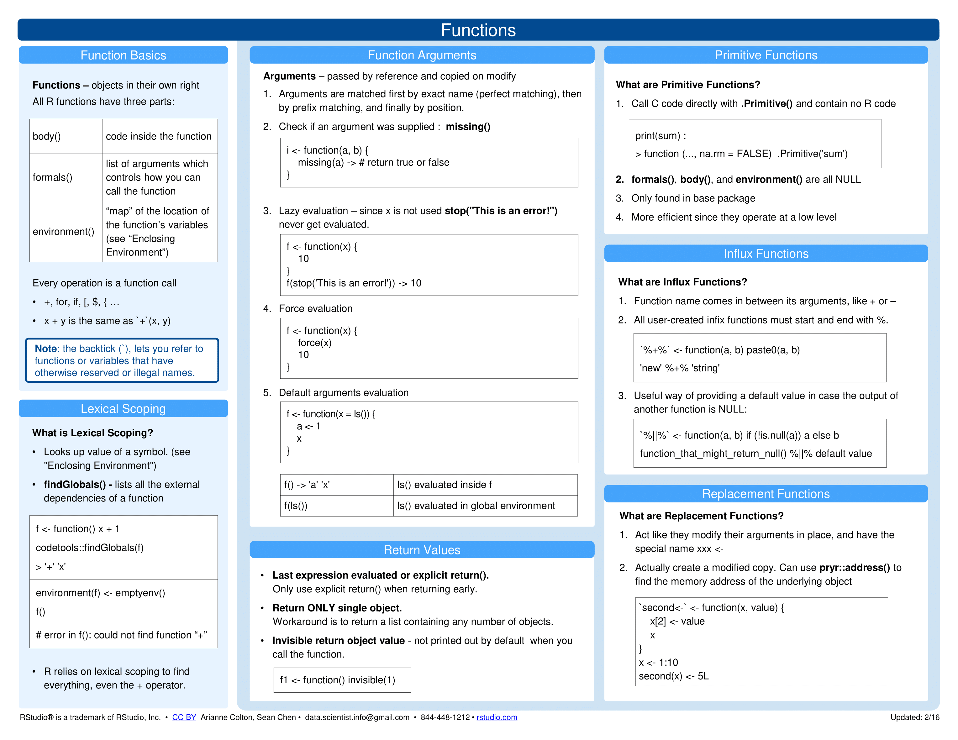
Figure 5.1: Summary on functions from the RStudio cheatsheet on Advanced R.

Chapters and books

The following chapters provide solid introductions to writing R functions:

• Chapter 19: Functions of the r4ds book (Wickham & Grolemund, 2017)

• Chapter 25: Functions (of the 2nd edition) of the r4ds book (Wickham, Çetinkaya-Rundel, et al., 2023)

More advanced aspects of functions are covered in:

• Section 11.4 of the ds4psy textbook (Neth, 2023a) and the set of corresponding exercises (in Section 11.7)

• Advanced R (Wickham, 2019) is a highly recommended resource for learning more about programming in R

See Section 11.6: Resources of the ds4psy book (Neth, 2023a) for additional resources.

5.5.3 Preview

The next Chapter 6 introduces iteration for executing code repeatedly.

5.6 Exercises

The first five of the following exercises are simple problems from 11.6: Exercises of the ds4psy book (Neth, 2023a):

5.6.1 Fun with errors

• Exercise 1

5.6.2 Conditional feeding

• Exercise 2

5.6.3 Buggy number recognition

• Exercise 3

5.6.4 Double standards?

• Exercise 4

5.6.5 Randomizers revisited

• Exercise 5

Here are some slightly more challenging exercises:

5.6.6 A comparison function

Create an as_logical() function that takes a vector x (e.g., x = 1:5), a comparison operator cop (e.g., cop = ">"), and a value val (e.g., val = 3) as inputs and returns the result of a logical test x cop val as its output (e.g., FALSE, FALSE, FALSE, TRUE, TRUE for 1:5 > 3).

Hint: Consider using switch() to distinguish between cases for possible comparison operators cop.

Note

A working as_logical() function is illustrated by the following examples:

# Check examples:
as_logical(x = 1:5, cop = ">=", val = 3)
#> [1] FALSE FALSE  TRUE  TRUE  TRUE
as_logical(c("A", "B", "C"), "!=", "A")
#> [1] FALSE  TRUE  TRUE
as_logical(c("A", "B", "C"), "in", c("A", "C"))
#> [1]  TRUE FALSE  TRUE

5.6.7 Extracting parts of a data frame

In this exercise, we will write some basic versions of existing data transformation functions (e.g., see the dplyr functions of Chapter 13):

1. Write a selection function my_select() that takes a data frame df and the names of variables (e.g., as a character vector of variable names) as inputs and returns the corresponding variables (or columns) of df as outputs.

2. Write a filter function my_filter() that takes a data frame df and a logical test on a variable as inputs and returns the cases (or rows) of df that satisfy the logical test as outputs. Hint: Use your as_logical() function (from above) to implement the logical test.

3. Combine the my_select() and my_filter() functions into a my_part() function that provides both functionalities in one function.

Note

Here are some snippets of code to create some testing data and check some functions that may be useful for solving the task:

# Create df: ------ 

N <- 10
df <- data.frame(name = LETTERS[1:N], 
                 age = sample(18:88, size = N, replace = TRUE), 
                 height = sample(150:200, size = N, replace = TRUE), 
                 team = sample(c("gym", "run", "swim"), size = N, replace = TRUE)
                 )
df

# Code snippets: ------ 

df_names <- names(df) 
vars <- c("name", "missing variable", "team", "xyz")

# select columns:
vars %in% df_names
df_names %in% vars

df[ , df_names %in% vars]  # logical indexing (columns of) df


# filter rows:
var <- "age"  # a variable in df
var_nr <- which(df_names == var)  # numeric index of a variable
v <- df[[var_nr]]                 # get corresponding vector

cond <- as_logical(v, "<", 40)    # result of test (using as_logical() from above)
df[cond, ]                        # logical indexing (rows of) df

Recursive functions

The following exercises involve recursive functions:

5.6.8 Improved factorials

1. Our recursive definition of fac(n) to compute \(n!\) (above) would fail for inputs of \(n\) that are not natural numbers (\(n \in \{1, 2, 3, ...\}\)). Add some initial verification steps to ensure that other cases (e.g., \(n = 0\), \(-1\), \(1/2\), or NA) are handled properly.

2. Our recursive definition of fac(n) to compute \(n!\) (above) works only for scalar inputs of \(n\). Generalize it to a fac_v() version that also works for longer vectors (i.e., length(n) > 1).

5.6.9 Reversing a vector

Task: Define a function reverse() that reverses the elements of a vector v (without using rev()).

Hint: A recursive version could use the case of a scalar vector v as a stopping criterion. The crux of a recursive reverse() function lies in its simplification step: Use c() and numeric indexing of v to place the first element at the end of the reversed rest of v.

#> [1] 5 4 3 2 1
#> [1] "C" NA  "A"
#> [1] NA

5.6.10 Recursive reading

A book can be viewed as a sequence of pages. For instance, a book containing 50 pages has pages that are numbered by \(1, 2, 3, ..., 50\). We can read the entire book by reading its first page, and then read the rest of the book (i.e., the remaining 49 pages), until the final page has been read.

1. Write a recursive read_book() function that can read any book that is defined as a sequence of consecutive page numbers (e.g., 1:50). The function should print out the current page number and print “the end” after reading the final page.

Hints: The recursive function should contain arguments for the current book and the current page number. The paste() function allows combining character and numeric objects, which can then be printed to the Console by the print() function.

2. Demonstrate that your read_book() function can read War & Peace, which contained \(1225\) pages in its 1st edition.

3. Check what happens when handling some special cases:

   • 1. Start reading on an intermediate page (e.g., on page 40).
   • 2. Read a book with page numbers have been arranged in a random order (using sample(book)).
   • 3. Combine a) and b).

This concludes our exercises on writing new functions. More advanced exercises on functions are provided in Section 11.7 of the ds4psy textbook (Neth, 2023a).