4 Conditionals

The current chapter covers conditional statements, which allow verifying data and distinguishing between cases to perform corresponding computations. In both spoken and computer languages, such constructs are typically signaled by “if-then” statements.

This chapter was originally placed after Chapter 5 on functions. But as functions often require conditionals, it makes more sense to cover conditionals before introducing functions.

Preparation

Recommended background readings for this chapter include:

Section 11.3: Conditionals of the ds4psy book (Neth, 2023a).
Section 19.4: Conditional execution of the r4ds book (Wickham & Grolemund, 2017).

Preflections

To reflect upon the notion and uses of conditionals, try answering the following questions:

Which types or linguistic variants of if-then do you know? (Hint: Think about necessary vs. sufficient conditions.)
What is the function of conditionals?
What feature of base R could serve similar functions? (Hint: Think about accessing R data structures.)

4.1 Introduction

Two roads diverged in a wood, and I,
I took the one less traveled by,
And that has made all the difference.

Robert Frost: The road not taken

One of the most basic types of decisions is choosing between options. The existence of diverging paths allows for a choice that will shape subsequent steps and thus make a difference. In programming, a more prosaic form of choice consists in distinguishing between cases: We often want to execute different lines of code depending on the type of current input or state (e.g., the value of some variable). Technical notions for this task are conditional execution or controlling information flow, but the simple motivation for those concepts is that we frequently need to check some criteria to make distinctions. In colloquial terms, conditionals typically involve some form of if-then statements.

The practical use of conditionals in programming can easily be seen: Demanding that some condition holds before executing some code allows for verifying data (e.g., ensure that some input has the right shape or type), and for distinguishing between cases (i.e., do this for one type of input, and something else for another). Together with the other constructs discussed in the chapters of this part, conditionals allow us to control and shape the flow of information in our code.

This chapter covers conditional execution in R in three sections:

Section 4.2 introduces basic if () else {} structures;
Section 4.3 introduces two more advanced conditionals: Using the vectorized ifelse() and the switch() function;
Section 4.4 discusses two alternatives to using conditionals in R: Using logical indexing/sub-setting and the cut() function.

Overall, we will learn how to use conditional structures in R, and how to avoid them by using alternative expressions.

4.2 Basic conditionals

The most basic commands for conditional execution in R are if and if-else constructs that resemble colloquial expressions. Syntactically, these statements use one the following structures:

if ( <condition> ) { <action> }
if ( <condition> ) { <action_1> } else { <action_2> }
if ( <condition_1> ) { <action_1> }
else if ( <condition_i> ) { <action_i> }
else { <action_n> }

Here, the word in <> describes the function of corresponding R expressions and the else if part (in c) can be repeated to distinguish an arbitrary number of cases. Note that the <condition> expressions are enclosed in (round) parentheses, whereas the <action> expressions are enclosed in curly brackets. We will briefly discuss these structures and explore some examples.

4.2.1 Features of `if () {}` conditionals

The general structure of conditional expressions in R is:

if ( <condition_i> ) { <action_i> } else { <action_n> }

To work properly, the expression in <condition_i> (in parentheses) must evaluate to a single logical value (i.e., either TRUE or FALSE). If a <condition_i> evaluates to TRUE, the following <action_i> (i.e., the corresponding then-part) is evaluated; otherwise (i.e., when the <condition_i> evaluates to FALSE), the alternative <action_n> (i.e., the corresponding else-part) is evaluated. The structure becomes more obvious when properly indending the code:

if ( <condition_i> ) { 
  <action_i>  # if condition_i is TRUE
} else { 
  <action_n>  # if condition_i is FALSE
}

The curly brackets {} around an <action> part are needed when action contains multiple expressions or extends over multiple lines of code. But even when not necessary, they help to visually structure expressions. Here are two simple examples of conditional expressions:

x <- -1

if (x < 0) {"x is negative"}
#> [1] "x is negative"

if (x > 0) {"x is positive"}

The 2nd example shows that — when <condition> evaluates to FALSE — the expression(s) in <action> are ignored. Sometimes we want to take an alternative action in this case. This can be achieved by adding an else part with a second <action_2> (again in curly brackets). A corresponding example is:

x <- 0

if (x < 0) {
  "x is negative"
} else {
  "x is non-negative"
}
#> [1] "x is non-negative"

Note two limitations of this if else structure:

The test of <condition> must evaluate to a logical scalar (i.e., either TRUE or FALSE).
The if else construct allows only for distinguishing between two cases.

The 2nd limitation can be overcome by adding conditional statements within cases. For instance, we could further distinguish the else case as follows:

x <- 0

if (x < 0) {
  
  "x is negative"
  
} else {
  
  if (x > 0) {
    
    "x is positive"
    
  } else {
    
    "x is zero"
    
  }
}
#> [1] "x is zero"

Note that using "x is zero" as the last <action> (in the final else part) avoided an explicit test for x being zero. If x is known to be assigned to an integer number, we could have used a condition (x == 0) for this purpose, but if x is computed elsewhere in our code, this may be error-prone (as a computed value of x may contain rounding errors and not evaluate to exactly zero). Note also lots of empty space — both horizontal indentation and vertical blank lines — renders the hierarchical structure of this conditional (and the 2nd conditional within the else part of the 1st conditional) transparent.

4.2.2 Adding cases by `else if () {}`

We can re-write our hierarchical (conditional within a conditional) construct into a more linear structure by inserting an additional else if () {} expression between the if and else parts of our original conditional:

x <- 0

if (x < 0) {
  
  "x is negative"
  
} else if (x > 0) {
  
  "x is positive"  
  
} else {
  
  "x is zero"
  
}
#> [1] "x is zero"

The general structure for this more flexible construct is:

if (condition_1) { 
  action_1     # if condition_1 is TRUE   
} else if (condition_i) {
  action_i     # if condition_1 is FALSE and condition_i is TRUE 
} else { 
  else_action  # if all previous conditions are FALSE
}

As this structure allows for an arbitrary number of else if parts (with corresponding pairs of <condition_i> and action_i), we can distinguish more than two cases in this way.

4.2.3 Conditional flow of control

How does R processes conditional expressions? As soon as R encounters a <condition> that evaluates to TRUE, R evaluates the corresponding <action> and then skips the rest of the conditional statement. This becomes important when two or more conditions are not mutually exclusive, as in the following example:

x <- 1001

if (x < 0) {
  
  "x is negative"
  
} else if (x > 0) {
  
  "x is positive"
  
} else if (x > 1000) {
  
  "x is a big number"
  
} else {
  
  "x is zero"
  
}
#> [1] "x is positive"

Given that the current value of x is 1001, the condition (x > 1000) would evaluate to TRUE. However, the condition is never reached, as the earlier condition (x > 0) also was TRUE and the corresponding <action> part was evaluated. Essentially, R evaluates a conditional expression only to the <action> of the first <condition> that evaluates to TRUE. In the extreme, this implies that R happily processes conditionals even when some conditions contain errors — as long as the inputs provided are all valid <condition> and <action> pairs:

x <- 1

if (x > 0){
  "x is pasitive"
} else {
  stop("ERROR")  # create an error
}
#> [1] "x is pasitive"

4.2.4 Multiple conditions

Finally, we can create more complex conditions by combining multiple <condition> statements into a logical structure (using the logical operators & or |). If so, either the combined <condition> must evaluate to a single logical value TRUE or FALSE, or a series of different conditions is linked with && or ||, which work like the logical connectors & and |, but are evaluated sequentially (from left to right). A corresponding example could take the following structure:

if (condition_1 || (condition_2 & condition_3)) { 
  "case 1"
} else { 
  "case 2"
}

Here, "case 1" would be printed as soon as condition_1 evaluated to TRUE, without considering the other conditions.

4.2.5 Practice

Write if (<condition>) {} else {} constructs to answer the following questions:
- What happens if the <condition> of an if else construct in R evaluates to more than one logical value?
- What happens if the <condition> of an if else construct in R evaluates to NA?

if (1 > 0:1) { "condition is TRUE" } else { "condition is FALSE" }
if (NA) { "condition is TRUE" } else { "condition is FALSE" }

Assuming that i is assigned to an integer, create a conditional that reports whether i is an even or an odd number. (Hint: The %% operator in an expression x %% y provides the remainder when dividing x by y.)
Create a conditional expression that reports whether an integer number i is divisible by 2, by 3, by both 2 and 3, or by neither 2 nor 3.
Describe the general conditions under which the following choices make a difference:
- linking logical conditions by & vs. &&
- linking logical conditions by | vs. ||

Then create examples that show the difference. (Hint: A difference due to serial evaluation can be demonstrated by including conditions that would yield an error, e.g., the stop() function.)

cond_1 <- TRUE
cond_2 <- stop()

if (cond_1 |  cond_2) { "ding" } else { "dong" } 
if (cond_1 || cond_2) { "ding" } else { "dong" } 

cond_1 <- FALSE

if (cond_1 &  cond_2) { "ding" } else { "dong" } 
if (cond_1 && cond_2) { "ding" } else { "dong" }

4.3 Advanced conditionals

To overcome some limitations of the basic if else structure, R provides more advanced conditional expressions. Two such structures introduced in this section are:

ifelse(<condition>, <action_1>, <action_2>) and
the switch() function.

4.3.1 Using `ifelse()`

A crucial limitation of R’s basic if (<condition>) {} else {} structure is that its <condition> must evaluate to a single truth value (i.e., to either TRUE or FALSE). However, when working with R data structures, we often deal with vectors of input values, rather than a single input value. For instance, we may have a vector v that is set to the integers from 1 to 5:

(v <- 1:10)
#>  [1]  1  2  3  4  5  6  7  8  9 10

A condition like v > 5 would evaluate to a logical vector:

v > 5
#>  [1] FALSE FALSE FALSE FALSE FALSE  TRUE  TRUE  TRUE  TRUE  TRUE

A corresponding conditional expression

if (v > 5) {"big"} else {"small"}

would yield an error, as the condition v > 3 fails to evaluate to a single logical value. In this situation, the vectorized ifelse() function allows to conduct as many logical tests as there are elements in v:

ifelse(v > 5, "big", "small")
#>  [1] "small" "small" "small" "small" "small" "big"   "big"   "big"   "big"  
#> [10] "big"

The general structure of such expressions is as follows:

ifelse(<condition>, <action_1>, <action_2>)

The superpower of ifelse() is that it works in an element-wise fashion: Each element of <condition> is assigned to either <action_1> or <action_2>, depending on the <condition> element evaluating either to TRUE or to FALSE, respectively. As a consequence, the output of the ifelse() function is an object of the same shape as <condition> (here: a vector of the same length).

When aiming to distinguish between more than two cases, we could compose hierarchical ifelse() statements that further distinguish between two versions of a case:

ifelse(v < 4, "small", ifelse(v > 7, "large", "medium") )
#>  [1] "small"  "small"  "small"  "medium" "medium" "medium" "medium" "large" 
#>  [9] "large"  "large"
ifelse(v > 7, "large", ifelse(v > 3, "medium", "small") )
#>  [1] "small"  "small"  "small"  "medium" "medium" "medium" "medium" "large" 
#>  [9] "large"  "large"

Note that the return values of the action_1, and action_2 parts of ifelse(<condition>, <action_1>, <action_2>) should typically be of the same type, and any NA values remain NA:

(v[c(4, 5, 7)] <- NA)  # add missing values to v
#> [1] NA
ifelse(v > 5, "big", "small")
#>  [1] "small" "small" "small" NA      NA      "big"   NA      "big"   "big"  
#> [10] "big"

Overall, ifelse() allows classifying a vector of values into two or more cases.

4.3.2 Using `switch()`

When aiming to distinguish many cases, the switch() function provides an alternative to overly complicated conditional statements. The basic structure of switch() is switch(EXPR, ...), where ... provides a list of alternatives. As the initial expression EXPR must either evaluate to either an integer or a text string (i.e., a character object), there are two ways to use switch():

If EXPR evaluates to an integer, the corresponding case in the list of alternatives ... is evaluated. An example of this case is:

# 1. switch() with a numeric EXPR:
number <- 3

switch(number,
       "one",
       "two",
       "three",
       "four")
#> [1] "three"

If EXPR evaluates to a character string, the alternatives of ... should be named and the alternative with a name corresponding to the character string is evaluated:

# 2. switch() with a character EXPR:
keyword <- "BB"

switch(keyword,
       "AA" = "one",
       "BB" = "two",
       "CC" = "three")
#> [1] "two"

This definition immediately raises two questions (corresponding to the integer and character versions, respectively):

What happens if an integer value is not within the number of cases?
What happens when there is no character string corresponding to the value of EXPR?

We can easily test this by adapting our examples:

# 1. switch() with a numeric EXPR:
number <- 10

switch(number,
       "one",
       "two",
       "three",
       "four")

# 2. switch() with a character EXPR:
keyword <- "XY"

switch(keyword,
       "AA" = "one",
       "BB" = "two",
       "CC" = "three")

Thus, if there is no case or keyword corresponding to the value of EXPR, switch() evaluates nothing (and returns a NULL object). Actually, the character case allows for an exception that answers a related question:

Can we specify a default or else case?

Only for the character version, a default or else case can be specified as follows:

# switch() with a character EXPR and default case:
keyword <- "XY"

switch(keyword,
       "AA" = "one",
       "BB" = "two",
       "CC" = "three", 
       "default/else case")
#> [1] "default/else case"

One last detail of switch() is that an empty list element corresponding to the name of EXPR will return the next non-empty element in .... This is harder to say than to see:

# switch() with a character EXPR and missing case:
keyword <- "BB"

switch(keyword,
       "AA" = "one",
       "BB" = ,
       "CC" = "three", 
       "default/else case")
#> [1] "three"

Overall, the switch() function is useful whenever a large number of cases is to be distinguished by an integer value or a verbal label.

4.3.3 Practice

Explain in which ways the ifelse() and switch() functions expand the basic functionality of the if-else conditional structure in R.
Re-write the conditional (from a practice task above) that reports whether i is an even or an odd number so that it works for a vector of integer inputs i.
Re-write the conditional (from a practice task above) that reports whether an integer number i is divisible by 2, by 3, by both 2 and 3, or by neither 2 nor 3, by using switch().

4.4 Alternatives to conditionals

In R, conditionals are often avoided or not needed, as we have other means of conditional execution. This section mentions two such alternatives to conditionals: Indexing or sub-setting and the cut() function.

4.4.1 Using logical indexing/sub-setting

In the preceding Chapters 2 and 3, we have been using an alternative to conditional expressions without always expressing it in these terms. When using logical indexing or sub-setting on vectors (in Section 2.3.3) or on (parts of) data frames (in Section 3.4.3), we chose and changed elements that satisfy some criterion. As we explicitly pointed out in Section 2.3.3, this can be interpreted as a conditional selection and transformation of data. To establish this insight more firmly, let’s use the following data frame df:

Table 4.1: Basic information on seven people.
name	sex	age	height
Adam	male	74	165
Bertha	female	18	170
Cecily	female	22	168
Dora	female	17	172
Eve	female	67	NA
Nero	male	29	185
Zeno	male	30	182

As an example, we can re-code the sex variable as a numeric gender variable.²² Before doing so, let’s first initialize it to a missing (or NA) value. Initializing new variables to NA values before re-coding the actual values is often a good idea, as we would notice any cases that got overlooked later:

# Initialize gender variable:
# df$gender <- rep(NA, length(df$sex))  # initialize variable
df$gender <- NA  # initialize variable

Suppose we wanted to set the value of gender as 1 when sex is “male”, and set it to 2 when sex is “female”. The following approach can often be observed in people who come from imperative programming languages (like SPSS), but would lead to an error in R:

# Erroneous conditionals:
if (df$sex == "male")   {df$gender <- 1}
if (df$sex == "female") {df$gender <- 2}

As the (<condition>) of an if statement in R must only evaluate to single logical value, this would fail. We could use the vectorized ifelse() expression (from above):

# Using ifelse():
(df$gender <- ifelse(df$sex == "male", 1, 2))
#> [1] 1 2 2 2 2 1 1

However, there is an even simpler solution that uses logical indexing or sub-setting of the df$sex vector. To demonstrate this, we initialize another gender_2 variable (to NA values) and assign the values 1 and 2 by logical indexing of the df$sex vector:

# Initialize new variable:
df$gender_2 <- NA

# Solution by logical indexing/subsetting: 
df$gender_2[df$sex == "male"]   <- 1
df$gender_2[df$sex == "female"] <- 2
df$gender_2
#> [1] 1 2 2 2 2 1 1

We can see that the values of the df$gender_2 variable correspond to the values of the df$gender variable:

# Verify equality of both solutions:
all.equal(df$gender, df$gender_2)
#> [1] TRUE

Thus, the two assignment operations (each with a logical index vector) to define df$gender_2 can replace the ifelse() operation to define df$gender (above). Actually, we have been using this alternative to conditional execution when re-coding the values of age and gender variables of a data frame (in Section @(struc:table)).

4.4.2 Using `cut()`

As another alternative to conditionals, the base R function cut() allows to categorize continuous data values into discrete bins. This is done by defining the breaks in the range of data values and assigning labels to the resulting categories.

As an example, suppose we wanted to categorize the age values of df into four categories “under 18” (ages up to 17), “young adult (ages from 18 to 29)”, “middle age (aged 30 to 64)”, and “senior (ages of 65+)”. Although we could accomplish this by a series of conditionals, we can also use the cut() function with an appropriate setting of its breaks argument:

df$age_cat <- cut(df$age,
                  breaks = c(-Inf, 18, 30, 65, +Inf), 
                  labels = c("under 18", "young adult", "middle age", "senior"), 
                  right = FALSE)
df$age_cat
#> [1] senior      young adult young adult under 18    senior      young adult
#> [7] middle age 
#> Levels: under 18 young adult middle age senior

The values of breaks define our category boundaries, with -Inf and +Inf generously specifying the minimum and maximum age values. The logical value of right determines whether the intervals specified by breaks should be closed on the right and open on the left (for right = TRUE), or vice verso (for right = FALSE). The resulting age_cat variable maps our age values into four categories:

Table 4.2: Result after using cut() to categorize continuous age values.
Name:	Age:	Age category:
Adam	74	senior
Bertha	18	young adult
Cecily	22	young adult
Dora	17	under 18
Eve	67	senior
Nero	29	young adult
Zeno	30	adult

Note that the cut() function created a factor variable with levels that were being defined by labels. (Chapter 16 provides additional information on factors.)

4.5 Conclusion

When you come to a fork in the road, take it.

Yogi Berra

This chapter introduced only a few new functions, but opened the door to programming in R. Our initial quote by Robert Frost emphasized that conditionals (or diverging roads) are difference makers. This insight translates into programming, as conditional statements allow for different paths that depend on the data values examined in their conditions. A more mundane aspect of working with conditionals can be derived from Yogi Berra’s tongue in cheek advice: Rather than fearing choices or avoiding conditionals, let’s embrace and use them productively in our analyses.

4.5.1 Summary

Conditionals allow us to verify data and to distinguish between cases, so that different inputs can receive different treatments.

In R, basic conditionals are available by using the simple if () {} or if () {} else {} templates.
The ifelse() function provides a version of conditionals that works for vectors, and the switch() function allows to distinguish between a large number of cases.
Many conditionals can be avoided by using logical indexing / sub-setting on data structures or by using the cut() function.

4.5.2 Resources

The resources noted in Chapter 3 also provide information on conditional expressions (and alternatives) in R:

Books and chapters

Cheatsheets

Here are some pointers to related Posit cheatsheets:

On base R:

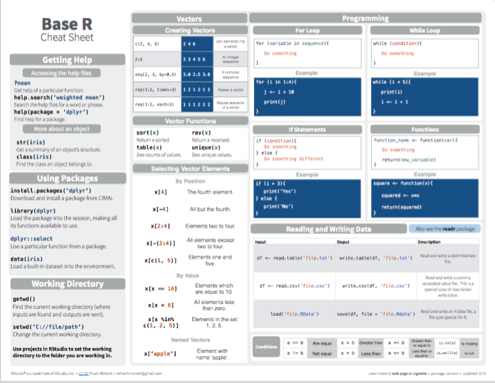
Figure 4.1: Base R summary from Posit cheatsheets.

More advanced aspects of R:

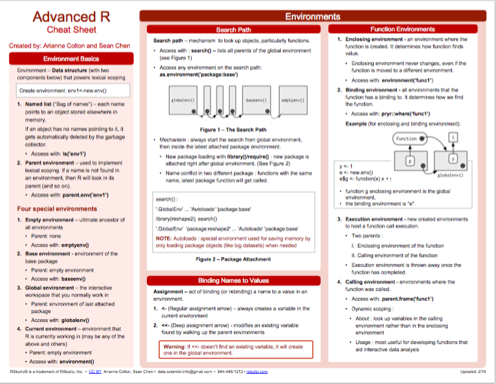
Figure 4.2: Advanced R summary from Posit cheatsheets.

4.5.3 Preview

The next Chapter 5 will teach us how to create our own functions.

4.6 Exercises

4.6.1 Verifying data types

The following questions refer to the evaluating of the size of the number x (in Sections 4.2 and 4.3 above):

Before categorizing the size of x, add an initial check that verifies that x is a number.
Create a conditional expression that tests for and reports the data type of an R object x.
Will the conditional statement of 2. be needed in R? Why or why not?

4.6.2 Vectorized `ifelse()`

Predict, evaluate, and explain the results (i.e., data types, shapes, and values) of the following expressions:

ifelse(1:4 > 0, "positive", FALSE)
ifelse(1:4 < 0, "negative", FALSE)
ifelse(1:4 > 2, "big", FALSE)
ifelse(1:4 > 2, c("yes", "yeah"), c("oh", "no"))
ifelse(1:2 == c(4, 2, 1, 2), c("A", "B", "C"), c("X", "Y"))

Hint: The terms atomic, vector and recycling should occur in the explanation.

4.6.3 Conditional greetings

Create a conditional expression that uses a scalar of the current hour (as an integer from 1 to 12) and of day_half (as a character object set to either “am” or “pm”) to provide one of the following greetings (at the appropriate value of hour):

“Good morning”
“Mahlzeit!” (i.e., German for “enjoy your lunch!”)
“Good afternoon”
“Good evening”
“Good night”

Note: Most people interpret “12pm” as noon and “12am” as midnight.

Solution

A possible solution could assign greetings to time values as follows:

Table 4.3: Example of possible greetings at different time values.
Time	Greeting
1am	Good night
4am	Good night
5am	Good morning
11am	Good morning
12pm	Mahlzeit!
1pm	Good afternoon
6pm	Good evening
10pm	Good night
12am	Good night

4.6.4 Conditional temperatures

Assume that we have a temperature value t (measured in degrees Celsius, with values ranging from $-50$ to $+50$) and we want to classify this value into common-sense categories (e.g., unbearably cold, freezing, cold, moderate, warm, hot, etc.).

Write a conditional expression (using an if-then-else construct) to categorize a scalar t value.
Re-write your conditional expression so that t could be a vector of multiple values (using ifelse()).
Re-write your conditional using the switch() function.
Re-write your conditional using the cut() function.

4.6.5 Conditional survey age

Re-solve 1.8.7 Exercise 7 of the ds4psy book (Neth, 2023a) by using conditional expressions (rather than logical indexing).

Whereas a realistic dataset would require non-binary gender values, two values are sufficient for our small sample.↩︎

Part 2: Programming basics

5 Functions