6 Iteration
Having learned how to use conditionals (in Chapter 4) and how to write functions (in Chapter 5), this chapter will introduce the notion of iteration, which means to repeatedly execute a process. As R is a functional programming language, the notion of iteration is deeply embedded in its DNA. Iteration in R can be explicit (by enclosing code in loops), but remains often implicit (by computing operations over vectors or applying functions to data structures).
This chapter concludes Part 2 on programming basics in R.
Preparation
Alternative introductions to iteration include:
Chapter 12: Iteration of the ds4psy book (Neth, 2025a).
Chapter 21: Iteration of the r4ds book (Wickham & Grolemund, 2017) or Chapter 26: Iteration in its 2nd edition (Wickham, Çetinkaya-Rundel, et al., 2023) for a tidyverse-centric perspective.
Preflections

To reflect upon the notion and uses of iteration, try answering the following questions:
What does the word iteration mean?
Why and when do we want to execute code repeatedly?
What other means of repeating code have we encountered in R?
6.1 Introduction
‘Begin at the beginning,’ the King said gravely,
‘and go on till you come to the end: then stop.’Lewis Carroll: Alice’s Adventures in Wonderland (Chapter XII)
The king’s instruction is so general that it may seem vacuous. Nevertheless, it aptly describes what happens when a human or a computer executes a rule-based process. But rather than moving straight from the beginning to the end, a characteristic feature of many computer programs is that they execute code in an iterative fashion.
The Latin term iter means “route”, and to “re-iterate” something is to repeat something. In ordinary language, proceeding in an “iterative” fashion typically means to proceed step-by-step until a goal has been achieved or some end has been reached.
In programming contexts, the term iteration means to repeat a process or procedure. However, unless this process or procedure includes some random element, strict repetition of a deterministic sequence of steps would only yield the same outcome. To be useful, we typically do not want to repeat an exact series of calculations, but handle different data inputs in each repetition. If the overall problem can be decomposed into many similar sub-problems, successfully solving each sub-problem helps to solve the overall problem.
Just as we have previously emphasized for functions (in Section 5.1), iteration provides a means of abstraction: By encapsulating a process (e.g., in a loop), we view it as a unit that we can repeat. As we can treat a loop as a black box that is defined in terms of its inputs and outputs, iteration and functions are closely related. Rather than constructing a loop, we could usually write a corresponding function and call this function repeatedly (but with different inputs).
In R, we can distinguish between explicit and implicit iteration. Explicit iteration involves loop structures (Section 6.2), whereas implicit iteration applies or maps functions to data structures (Section 6.3).
6.2 Explicit iteration: Loops
Loops are structures of code that cause some code (i.e., a collection of R expressions) to be executed repeatedly. The series of expressions or loop <body> to be repeated is enclosed in curly brackets { <body> }. To instruct R when and how often the <body> is to be evaluated, any loop requires some condition or criterion that indicates whether to continue with another iteration or to stop and exit the loop.
Explicit loop types
R provides three basic structures for explicit iteration:
forloops define an explicit index variable and the range of values that this variable should assume. They are indicated when we know (or can determine) the number of required iterations in advance.whileloops are more general and specify the condition for repeating a process. They are indicated when we primarily know a condition that should end a loop.repeatloops re-iterate a process until abreakkeyword is encountered. They are similar towhileloops, but require an explicit termination signal.
Loop keywords
When defining explicit loops, two keyword constructs provide additional control over the flow of information:
nextabandons the<body>of the current loop iteration and begins the next iteration of the same loop.breakcauses an exit from the<body>of the current (innermost) loop and continues with the code after this loop.
We will discuss these types of loops and keywords in the following sections.
6.2.1 for loops
The general structure of a for loop in R is as follows:
In this template, i is an index variable that assumes a new value for every iteration of the loop, <seq> denotes the sequence of values of i, and <body> can be an arbitrary series of R expressions.
Note that defining seq (e.g., as 1:n) implies that the number of repetitions n is known or can be determined (e.g., from the shape of some data structure).
To be helpful, the loop <body> must either evoke desired side effects (e.g., print or plot something) or modify some data structure that collects the results. If the current overall (or global) problem can be decomposed into many (local) sub-problems, solving each sub-problem and storing its solution in some data structure helps to solve the overall problem.
Before writing a for loop, we first must figure out its range and the type of output we need or want. Correspondingly, two key questions for creating a for loop are:
Which range: Over which variable and range of values do we want to iterate (to construct
<seq>)?Which output: How do we provide the local results of each loop iteration or collect them to answer our global problem?
A loop recipe
A general recipe for creating loops includes the following steps:
Decompose an overall problem into many similar sub-problems.
Anticipate the desired output of each sub-problem and prepare a data structure to collect this output.
Define an index variable
i, a sequence<seq>, and a loop<body>that solves each sub-problem and collects its result in the output.Use the loop output to solve the overall problem.
In the following, we illustrate this recipe for simple examples.
Using for loops
To illustrate the creation of loops (and later the application of functions), we first create a simple data structure.
Here is a data frame df, that contains the numbers from 1 to 20 in 5 rows and 4 columns, with its variables named A to D:
df        <- data.frame(matrix(1:20, ncol = 4, byrow = TRUE))
names(df) <- LETTERS[1:4]
df
#>    A  B  C  D
#> 1  1  2  3  4
#> 2  5  6  7  8
#> 3  9 10 11 12
#> 4 13 14 15 16
#> 5 17 18 19 20
Our goal for various loops in this chapter will be to compute arithmetic results (e.g., the sum, mean, etc.) over the rows and columns of this data. Although this helps to illustrate the creation of loops, we emphasize that we usually do not need loops for solving such simple tasks. For instance, there even exist R functions for computing the sum of (numeric) rows or columns:
But if we were ignorant of these functions (or had to solve tasks that lack a dedicated function), a general strategy for solving such tasks consists in using a for loops to derive and collect the desired results.
Sums of rows
We can apply our general loop recipe to the current overall problem (of computing the row sums of a data frame):
Decomposition: We obtain the row sums of a data frame
dfby computing the sum of each individual row.Expected output: We expect to obtain a vector of numeric sums and initialize
outas 5 missing values.Design loop: We define a
forloop that increments an index variableifrom 1 tonrow(df). The loop<body>must sum the values of each row and collect them inout.Use output: As our solution to the overall problem, we simply print
outto view the computed row sums.
# A. Prepare data structure to store output:
out <- rep(NA, nrow(df))

# B. Create for loop:
for (i in 1:nrow(df)){

  # a. Type the name of each variable (specific, but inflexible):
  out[i] <- df$A[i] + df$B[i] + df$C[i] + df$D[i]

  # b. Sum the i-th row of df (better, as more general):
  out[i] <- sum(df[i, ])

}

# C. Use output:
out  # print
#> [1] 10 26 42 58 74
Note that we implemented two different solutions in the <body> of our loop:
Variant a. refers to each variable (column) of
dfby its name and explicitly adds the corresponding values. This solution requires typing each variable name, but could also handle data frames with non-numeric columns.Variant b. uses numerical indexing of
dfto select each row ofdfand adds their values by thesum()function. This solution works when all values are numeric.
Both variants yield the same solution (which is why we could keep both of them), but b. is more flexible and elegant than a (as long as all columns are numeric).
In this example, solving the overall problem only consisted in printing the solutions stored in out. But in real applications we would probably continue doing other things with them.
We can verify that we obtained the expected sums by comparing the values of out with the corresponding results of the rowSums() function:
Sums of columns
Given that our data frame df consists only of numbers, summing its rows and columns seems very similar. However, knowing that a data frame stores variables (or vectors) in columns, rather than in rows, suggests that both directions may not be quite so similar.
However, we can solve the overall problem of computing all column sums of df with a for loop by making only minimal changes (changing the definition of <seq> from nrow() to ncol() and indexing the 2nd dimension of df in the loop <body>):
# A. Prepare output:
out <- rep(NA, ncol(df))

# B. Create for loop:
# for (i in 1:ncol(df)){   # explicit <seq> range
for (i in seq_along(df)){  # implicit <seq> range

  out[i] <- sum(df[ , i])  # i-th column

}

# C. Use output:
out
#> [1] 45 50 55 60
In defining the range <seq> of this for loop, we also replaced the explicit value range definition (as a numeric vector 1:ncol(df)) by the seq_along() function.
When the range of loop values can be determined by a data structure, seq_along() allows to define the value range in a more implicit fashion.
Its output depends on its type of input:
When used on a vector v, seq_along(v) returns a vector of integers from 1 to length(v).
When used on a data frame df, seq_along(df) returns an integer vector of the column numbers (i.e., the indices of the list elements of df).
Again, let’s verify that out contains the same result as the corresponding function:
Thus, our second for loop also yielded the same results as the corresponding function.
Let’s practice our knowledge and skills on for loops before we study while and repeat loops.
Practice
Create
forloops for computing the row and column means and medians ofdf.What would change, if we added
nextas the last statement of a loop’s<body>? What would change, if we addedbreakas the last statement of a loop’s<body>? (Predict and then try out both in your solutions to 1.)It seems that
1:nandseq_along(1:n)yield identical results. Explain the difference between them and whyseq_along()still makes sense.
Solution
# Yes:
all.equal(1:5, seq_along(1:5))
#> [1] TRUE
# but only because each element in the vector 1:5 corresponds to the
# (numeric index of the) i-th element of 1:5 (which is what seq_along(v) provides).

# Differences between v and seq_along(v) are far more common:
all.equal(5:1, seq_along(1:5))
#> [1] "Mean relative difference: 1"
all.equal(runif(5), seq_along(runif(5)))
#> [1] "Mean relative difference: 4.434031"
all.equal(letters[1:5], seq_along(letters[1:5]))
#> [1] "Modes: character, numeric"
#> [2] "target is character, current is numeric"

# seq_along() is more general than 1:n:
# seq_along() corresponds to 1:length(v) for vectors v.
# seq_along() corresponds to 1:ncol(df) for data frames df. - How could the
forloops that iterate over all rows ofdfbe re-written withseq_along()?
Solution
By using seq_along() for a vector (i.e., a column) of df (e.g., df[, 1] or df[[1]]).
- Use a
forloop to write a function that computes the factorial \(n!\) (for a non-negative integern).
Hint: The factorial \(n!\) is also computed by the base R function factorial() and was previously defined as a recursive fac() function (in Section 5.4.3).
Solution
The most complicated parts of the following fac_for() function are the conditionals to catch some special cases.
By contrast, the for loop to multiply fac by each number i is simple:
fac_for <- function(n){

  # Catch some special cases:
  if (is.na(n) || is.character(n) || n < 0) { return(NA) }
  if (!ds4psy::is_wholenumber(n)) { stop("n must be an integer >= 0") }

  fac <- 1  # initialize output

  for (i in 1:n){

    fac <- i * fac

  }

  return(fac)

}
After handling some special cases (by an early return() and a stop() function), we initialize an output variable fac to a value of 1.
Next, we set up the loop <seq> to iterate over 1:n.
The loop <body> consists of a single line that updates the value of fac to the product i * fac.
After the loop and at the end of the function, we return the current value of fac.
Let’s check our fac_for() function for some scalar inputs:
# Check:
fac_for(NA)
#> [1] NA
fac_for(-1)
#> [1] NA
fac_for(3/2)
#> Error in fac_for(3/2): n must be an integer >= 0
fac_for(0)
#> [1] 0
fac_for(1)
#> [1] 1
fac_for(2)
#> [1] 2
fac_for(10)
#> [1] 3628800

all.equal(fac_for(123), factorial(123))
#> [1] TRUE
This suggests that fac_for() works as intended, as long as we only provide scalar inputs for n.
However, note that the for loop was not really necessary to solve this task.
An even simpler solution could directly compute the product of the vector elements 1:n:
fac_prod <- function(n){

  # Catch some special cases:
  if (is.na(n) || is.character(n) || n < 0) { return(NA) }
  if (!ds4psy::is_wholenumber(n)) { stop("n must be an integer >= 0") }

  return(prod(1:n))

}

# Check:
fac_prod(NA)
#> [1] NA
fac_prod(-1)
#> [1] NA
fac_prod(3/2)
#> Error in fac_prod(3/2): n must be an integer >= 0
fac_prod(0)
#> [1] 0
fac_prod(1)
#> [1] 1
fac_prod(2)
#> [1] 2
fac_prod(10)
#> [1] 3628800

all.equal(fac_prod(123), factorial(123))
#> [1] TRUE
In addition to for loops, the second construct of explicit iteration in R is a while loop.
6.2.2 while loops
The structure of a while loop seems even simpler than a for loop because it only has two components, a <condition> and a <body>:
However, this structural simplicity is deceiving, as it hides requirements on both the <condition> and the <body> of the loop.
To execute the <body> of a while loop, its <condition> must initially evaluate to TRUE.
More importantly, to ensure that the while loop eventually stops, its <body> must contain code that eventually changes the <condition> from TRUE to FALSE.
A while loop is somewhat more general than a for loop, as any for loop can easily be written as a while loop, but not necessarily vice versa.
For instance, a for loop with n steps:
can be re-written as a while loop that uses a counter variable i for the number of iterations and a condition that some maximum number of steps n must not be exceeded:
As while loops require some explicit maintenance (here: the initialization and incrementation of a counter), we prefer using for loops when the number of iterations is available in advance. However, we often cannot know in advance how many iterations we will need — and that’s what while loops are for.
Using while loops
As an example of a while loop use case, let’s throw two fair coins until we obtain two heads (denoted by the character "H", whereas the alternative outcome tails is denoted by "T") at once.
As we do not know how long this will take, we throw our coins in a while loop and always check the results for our target event:
Here is a basic version of a while loop that runs until the desired event occurs:
# Initialize:
two_heads <- FALSE

while (!two_heads) {

  # Throw coins:
  cur_throw <- sample(c("H", "T"), size = 2, replace = TRUE)

  # Feedback (on Console):
  cat(cur_throw, "\n", sep = "")

  # Stopping criterion:
  if (all(cur_throw == "H")) {
    two_heads <- TRUE
  }

}
#> TH
#> TH
#> TH
#> TT
#> TT
#> TH
#> TT
#> HH
The cat() function concatenates and prints the character vector cur_throw (and \n is a special new line character).
Our task gets trickier when we also want to collect the intermediate results.
Lacking a given counter variable i, we can explicitly create one and increment it each time the loop is being executed.
Additionally, we create an all_throws vector that will store our results.
However, since we do not know the number of iterations, we can only initialize it to a scalar and then assign current events to the i-th element of all_throws:
# Initialize:
two_heads  <- FALSE
all_throws <- NA
i <- 0

while (!two_heads) {

  # Increment counter:
  i <- i + 1

  # Throw coins:
  cur_throw <- sample(c("H", "T"), size = 2, replace = TRUE)

  # Feedback (on Console):
  cat(i, ": ", cur_throw, "\n", sep = "")

  # Collect results:
  all_throws[i] <- paste(cur_throw, collapse = "")

  # Stopping criterion:
  if (all(cur_throw == "H")) {
    two_heads <- TRUE
  }

}
#> 1: TT
#> 2: TT
#> 3: HT
#> 4: TH
#> 5: HT
#> 6: TH
#> 7: HH

# Output:
all_throws
#> [1] "TT" "TT" "HT" "TH" "HT" "TH" "HH"
This works, but increasing the length of all_throws vector on each iteration is not a good idea. An alternative that may be faster is to initialize cur_throw to a longer vector. In the current example, we can estimate that the random target event should occur on every four iterations on average, but randomness can require many more throws with low, but non-negligible probabilities.
6.2.3 repeat loops
A repeat loop is even more general than a while loop:
It continues to iterate through the loop <body> until the stop signal break is encountered. Its general structure is:
Actually, a repeat loop is very similar to a while loop:
Just as we need to ensure that the <condition> of while eventually switches from being TRUE to being FALSE, a repeat loop must ensure that some <condition> eventually turns TRUE so that encountering break exits the loop.
Both loop types risk getting lost in infinite looping, unless some event actually occurs and causes an exit.
The key difference is that a repeat loop explicitly encodes the break, whereas a while loop leaves the break implicit in the truth value of its <condition>.
Using repeat loops
To illustrate a repeat loop, we move from flipping coins to rolling dice.
Let’s roll a pair of dice (each showing numbers from 1 to 6) until a combination of 1 and 2 is being rolled (a compound event known — at least in parts of Germany — as a “Mäxle”).
The word “until” signals that we cannot know how many iterations this will require.
Hence, we use a repeat loop that repeats a process until our goal is reached:
repeat {

  dice <- sort(sample(1:6, size = 2, replace = TRUE))

  print(dice)

  if ((dice[1] == 1) & (dice[2] == 2)) {
    break # required
    }

  next  # optional

}
#> [1] 2 4
#> [1] 2 5
#> [1] 4 5
#> [1] 5 5
#> [1] 1 5
#> [1] 1 6
#> [1] 1 2
Note that the use of sort() to arrange the numeric outcomes of sample() in ascending order facilitates our stopping condition (as it ensures that the first element of dice must be a 1 and the 2nd must be 2, rather than also checking the opposite order).
As we have emphasized for white loops (above), it is crucial that the stopping condition of our repeat loop will eventually evaluate to TRUE, so that the break keyword is encountered. Otherwise, the loop would repeat eternally — or until some external force (or a lack of electrical power) terminates it.
The core requirement of loops is that decomposing an overall problem into many similar sub-problems helps solving the overall problem. As we will see in the next section on implicit iteration (in Section 6.3), there are (usually) easier and smarter ways for addressing iterative tasks than using explicit loops. But whereas there may be more elegant ways of solving the simple tasks for which we have created loops so far, the general notion of loops can also solve problems for which there exist no dedicated functions. And although loops are often denounced as somewhat clumsy or slow in R, there is nothing wrong with being explicit about an iteration.
Practice
Before we move on from explicit to implicit iteration, let’s practice while and repeat loops:
- Write a
whileand arepeatloop that throws three fair coins (each with an outcome of either “H” or “T”) until all three show the same outcome. Ensure that the loop outputs provide both the exact sequence of the obtained outcomes and the number of iterations needed to solve the problem.
Hint: When storing all outcomes in a suitable data structure, its shape represents the number of iterations.
Re-write our example of a coin flipping
whileloop (from above) as aforloop that allows for a large number of iterations (e.g.,for (i in 1:1000)and abreakkeyword). What are the advantages and disadvantages offorvs.whileloops?Re-write our example of a dice rolling
repeat`` loop (from above) as awhileloop and aforloop that allows for a large number of iterations. What are the advantages and disadvantages ofrepeat`vs.\whilevs.\for` loops?
6.3 Implicit iteration: Functional programming
Implicit iteration is a key competence of R — and something we already are familiar with.
For instance, many operations (e.g., arithmetic ones) are vectorized in R, so that we do not need to use a loop (e.g., to multiply a vector v by a scalar constant c).
As a consequence, explicit iteration is not as common in R as it is in most other programming languages. And when a loop primarily traverses or modifies a data structure, it is possible to replace explicit loops by wrapping up their <body> in a function, and then repeatedly apply that function to the data.
In Chapter 5, we saw that functions provide a way of abstracting and encapsulating a series of instructions: Instead of writing a loop, we can enclose the required code in a function and then call this function repeatedly. As R provides sophisticated ways of repeatedly applying functions to data structures, it is known as a functional programming language.
In Section 2.2, we cited:
To understand computations in R, two slogans are helpful:
- Everything that exists is an object.
- Everything that happens is a function call.John Chambers
A superficial reading of this statement could mis-interpret it as suggesting a division between (or dichotomy of) objects and functions.
However, in Chapter 5, we have seen that functions are objects that are defined like other objects (by assigning the output of the function() function to an object name).
Now it is time to break down another barrier between two seemingly distinct concepts:
That between data and functions.
As we will see, R provides several ways of avoiding explicit loops and these ways work by using functions as data arguments that are being passed by functions.
Whereas most beginners find the abstract notion of implicit iteration (i.e., applying functions to data structures) difficult to grasp, it is actually simpler than many explicit loops.
As we focus on the essentials in this book, we only briefly introduce the base R apply() (R Core Team, 2025a) and purrr’s map() family of functions (Wickham & Henry, 2026).
6.3.1 Applying functions to data structures
R provides a family of functions for implicit looping (e.g., apply(), lapply(), and tapply()).
They all have in common that they take some data structure X and the name of some function FUN as inputs and provide some output after applying FUN to X.
They differ in the data structures for inputs and outputs, and which other arguments they allow for.
In Section 6.2 above, our first two examples of for loops computed the row and column sums of some data frame df:
# Data structure (from above):
df
#>    A  B  C  D
#> 1  1  2  3  4
#> 2  5  6  7  8
#> 3  9 10 11 12
#> 4 13 14 15 16
#> 5 17 18 19 20

# Solutions:
rowSums(df)
#> [1] 10 26 42 58 74
colSums(df)
#>  A  B  C  D
#> 45 50 55 60
Rather than defining explicit loops that solve this task, we will now solve it with implicit iteration.
Using apply()
Given that we have the sum() function to compute the sum (of a numeric vector), it would be nice to instruct R to apply this function to each row of the data structure df.
The apply() function does exactly this:
apply(X = df, MARGIN = 1, FUN = sum)
#> [1] 10 26 42 58 74
Note that the arguments of apply() require some data (X = df), a function to be applied (FUN = sum), and some detail how the function should be applied to the data.
This detail is provided by the MARGIN argument.
For a rectangular data structure (e.g., a matrix or data frame), MARGIN specifies the dimension over which FUN should be applied to X:
A value of 1 denotes rows, whereas 2 denotes columns.
Thus, we can easily obtain the result of our 2nd for loop from Section 6.2 above, which computed the column sums of df:
apply(X = df, MARGIN = 2, FUN = sum)
#>  A  B  C  D
#> 45 50 55 60
Note that we passed the name of the sum() function as a data argument of apply().
From studying the documentation of apply() (by evaluating ?apply), we can learn that — in addition to three required arguments X, MARGIN and FUN — it also allows for optional arguments (...) to be passed to FUN.
For instance, if our data had contained any missing values, we could have added the argument na.rm = TRUE to be passed to the sum() function (to only add all non-missing values).
Equipped with the power to apply functions to data, we can avoid many explicit loops.
Instead, tasks like the first Practice task above (which asked to compute the row and column means and medians of df) can be immediately be solved by applying suitable functions to our data structure.
Using lapply()
To deal with different data structures, base R also provides several variants of apply(). The lapply() function applies a function FUN to a list X and returns a list of the same length as X.
Each element of the returned list is the result of applying FUN to the corresponding element of X.
To provide some examples, we can define a list ls as follows:
ls <- list(a = 1L:10L,
           b = seq(-1, +1, by = 1/2),
           c = c(TRUE, FALSE, FALSE, TRUE)
           )
ls
#> $a
#>  [1]  1  2  3  4  5  6  7  8  9 10
#>
#> $b
#> [1] -1.0 -0.5  0.0  0.5  1.0
#>
#> $c
#> [1]  TRUE FALSE FALSE  TRUE
Although the elements of this list are vectors of different length and type,
we can compute the sum() or mean() of each list element by:
# Apply FUN to list elements:
lapply(X = ls, FUN = sum)
#> $a
#> [1] 55
#>
#> $b
#> [1] 0
#>
#> $c
#> [1] 2
lapply(X = ls, FUN = mean)
#> $a
#> [1] 5.5
#>
#> $b
#> [1] 0
#>
#> $c
#> [1] 0.5
Actually, since a data frame also is a list of vectors (see Chapter 3), we can compute the column sums of df (computed explicitly by a for loop and implicitly by apply(df, MARGIN = 2, FUN = sum) above) alternatively by:
# Apply FUN to data frame variables (columns):
lapply(X = df, FUN = sum)
#> $A
#> [1] 45
#>
#> $B
#> [1] 50
#>
#> $C
#> [1] 55
#>
#> $D
#> [1] 60
As lapply() not only accwepts list inputs, but also returns its output as the elements of a list, it can be maximally flexible.
For instance, if the function denoted by FUN returns more than one value as its output, lapply() can still cope with them:
# Apply FUN to data frame variables (columns):
lapply(df, range)
#> $A
#> [1]  1 17
#>
#> $B
#> [1]  2 18
#>
#> $C
#> [1]  3 19
#>
#> $D
#> [1]  4 20
lapply(df, quantile)
#> $A
#>   0%  25%  50%  75% 100%
#>    1    5    9   13   17
#>
#> $B
#>   0%  25%  50%  75% 100%
#>    2    6   10   14   18
#>
#> $C
#>   0%  25%  50%  75% 100%
#>    3    7   11   15   19
#>
#> $D
#>   0%  25%  50%  75% 100%
#>    4    8   12   16   20
Despite the unmatched flexibility of lists, we often would prefer non-list outputs, which is where sapply() comes into play.
Using sapply()
When we prefer simpler output formats to lists, we can replace lapply(X, FUN) by sapply(X, FUN) (where s stands for simplified).
Essentially, sapply() is a user-friendlier version of lapply() that returns its output as a named vector (if possible):
# Apply FUN to list elements (and simplify output):
sapply(X = ls, FUN = sum)
#>  a  b  c
#> 55  0  2
sapply(X = ls, FUN = mean)
#>   a   b   c
#> 5.5 0.0 0.5
For our data frame df, using sapply() to apply a function to each variable (column) simplifies the output to a named vector or a matrix (if needed):
# Apply FUN to data frame (and simplify output):
sapply(df, sum)       # as a vector
#>  A  B  C  D
#> 45 50 55 60
sapply(df, range)     # as a matrix
#>       A  B  C  D
#> [1,]  1  2  3  4
#> [2,] 17 18 19 20
sapply(df, quantile)  # as a matrix
#>       A  B  C  D
#> 0%    1  2  3  4
#> 25%   5  6  7  8
#> 50%   9 10 11 12
#> 75%  13 14 15 16
#> 100% 17 18 19 20
The apply() family of functions has even more members.
We will briefly introduce some of them, but see the documentations and examples of
vapply(), mapply(), rapply() and tapply() for more specialized and sophisticated versions of the apply() function.
vapply()
The vapply() function is similar to sapply(), but provides additional control over the shape and type of the output. Setting its FUN.VALUE to 1 returns a vector of length(X), otherwise an array that matches the structure of FUN.VALUE.
While this can be safer, using vapply() can require a lot of typing: vapply(df, is.numeric, logical(1)) provides its output as logical values (and is equivalent to purrr::map_lgl(df, is.numeric), see below).
mapply()
The mapply() function provides a multi-variate version of sapply().
Essentially, mapply(FUN, ...) applies FUN to the first elements of each ... argument, the second elements, the third elements, etc. Its ... argument accepts multiple arguments to vectorize over, which will be recycled to a common length.
tapply()
The tapply() function is probably the most impressive apply() member.
Its INDEX argument accepts a list of one or more factors (or a formula) that are applied to X.
This allows computing sophisticated aggregate summaries over combinations of data values for vectors or data frames. (The documentation of ?tapply() refers to these combinations as a “ragged array”, which essentially means that they can contain a variable number of elements.)
Here are some basic examples for applying tapply() to data structures:
- Summaries of vector values:
Given a vector of dice
throws:
# Data:
throws <- sample(1:6, size = 30, replace = TRUE)
throws
#>  [1] 5 2 4 2 1 6 2 3 6 3 2 4 5 1 3 4 3 3 4 5 6 1 3 2 5 4 4 5 5 3
we can use tapply() to compute summaries over their possible values:
# Summary of vector values:
tapply(X = throws, INDEX = throws, FUN = length)
#> 1 2 3 4 5 6
#> 3 5 7 6 6 3
table(throws)  # almost identical
#> throws
#> 1 2 3 4 5 6
#> 3 5 7 6 6 3
# but:
tapply(X = throws, INDEX = throws, FUN = sum)
#>  1  2  3  4  5  6
#> 3 10 21 24 30 18- Contingency tables (from data frames):
Given the datasets data
warpbreaks:
#> # A tibble: 54 × 3
#>    breaks wool  tension
#>     <dbl> <fct> <fct>
#>  1     26 A     L
#>  2     30 A     L
#>  3     54 A     L
#>  4     25 A     L
#>  5     70 A     L
#>  6     52 A     L
#>  7     51 A     L
#>  8     26 A     L
#>  9     67 A     L
#> 10     18 A     M
#> # ℹ 44 more rows
we can use tapply() to create summaries of variable levels/factor combinations:
# Contingency table from data.frame:
tapply(X = warpbreaks$breaks, INDEX = warpbreaks[ ,   2], FUN = sum)
#>   A   B
#> 838 682
tapply(X = warpbreaks$breaks, INDEX = warpbreaks[ , 2:3], FUN = sum)
#>     tension
#> wool   L   M   H
#>    A 401 216 221
#>    B 254 259 169

# Averages over groups:
tapply(warpbreaks$breaks, warpbreaks[ ,   2], mean)
#>        A        B
#> 31.03704 25.25926
tapply(warpbreaks$breaks, warpbreaks[ , 2:3], mean)
#>     tension
#> wool        L        M        H
#>    A 44.55556 24.00000 24.55556
#> B 28.22222 28.77778 18.77778- Averages over groups:
Let’s assume some dataset
pcgthat includes the initials of professors, their courses, and corresponding grades (for individuals students or assignements):
#> # A tibble: 100 × 3
#>    prof  course  grade
#>    <chr> <chr>   <int>
#>  1 C.D.  arts        3
#>  2 A.B.  arts        1
#>  3 B.C.  science     2
#>  4 B.C.  arts        3
#>  5 C.D.  arts        3
#>  6 C.D.  science     4
#>  7 B.C.  arts        1
#>  8 A.B.  science     1
#>  9 A.B.  data        4
#> 10 B.C.  data        2
#> # ℹ 90 more rows
we can use tapply() to compute the average grade over (combinations of) variable levels:
# Compute group averages:
tapply(pcg$grade, pcg$prof,    mean)
#>     A.B.     B.C.     C.D.
#> 2.371429 2.533333 2.285714
tapply(pcg$grade, pcg[ , 2],   mean)
#>     arts     data  science
#> 2.078947 2.545455 2.620690
tapply(pcg$grade, pcg[ , 1:2], mean)
#>       course
#> prof       arts     data  science
#>   A.B. 2.071429 2.833333 2.222222
#>   B.C. 2.000000 2.625000 2.916667
#>   C.D. 2.142857 2.230769 2.625000
rapply()
The rapply() function is a recursive version of lapply() with additional control over how the result is structured. The type of output is determined by the arguments how and classes. (See ?rapply() for its documentation and examples.)
Overall, the apply() family of functions provides a powerful toolbox for applying functions to data structures. However, the variety of function names and their (sometimes inconsistent) arguments make it difficult to map the family members to tasks and to master each function. In the likely case that you find the family of apply() functions confusing, you must not despair:
The *purrr package provides a similar range of functions in a more consistent way.
6.3.2 Mapping functions of purrr
The R package purrr (Wickham & Henry, 2026) contains a family of map() functions that provide updated and more consistent versions of apply().
The main goal of using purrr functions (instead of for loops) is to break common list manipulation challenges into smaller and independent pieces.
This strategy scales down the problem, solves its sub-problems, and then tries to solve the overall problem from those pieces:
Decomposing a complex problem into smaller sub-problems that allow us to advance towards a solution.
Solving the sub-problem for a single element of a list.
Constructing an overall solution from the sub-problem solutions.
Once we have solved the sub-problem, purrr takes care of generalizing the solution to every element in the list and construct an overall solution from those pieces.
The scaling-down and up-again strategy of purrr matches our general strategy for explicit iteration (above), but is implemented in more concise expressions. While this affords a greater level of abstraction, it also makes it easier to solve related problems and to understand the solutions to old problems when re-reading older code.
Essential map() functions
The pattern of looping over a vector, doing something to each element, and saving the results is so common that the purrr package provides a family of functions for it. To control the type of output, there is a separate function for each output type:
-
map()creates a list.
-
map_lgl()creates a logical vector.
-
map_int()creates an integer vector.
-
map_dbl()creates a double vector.
-
map_chr()creates a character vector.
Each of these functions takes a vector (or data frame) .x as input, applies a function .f to each element, and then returns a new vector whose length corresponds to (and has the same names as) the input vector. The type of the output vector is determined by the suffix _? of the map() function (e.g., map_chr() returns the output as a character vector).
Examples
The most common use of map() applies a function .f to each variable/column of a data frame .x. For instance, we can use map_dbl() on the data frame df (from above) to compute various statistical measures (with numeric doubles as output):
map() variants
Several variants of the map() function accommodate a different number of arguments:
-
map()applies a function.fto 1 argument.x
-
map2()applies a function.fto 2 arguments.xand.y -
pmap()applies a function.fto 3 or more arguments (provided as a list.l)
As before, typical uses of map_() specify the expected data type of the output as a suffix (after an underscore _).
Here is a numeric example that uses three different map() functions:
# Create data:
tb <- data.frame(n_1 = sample(1:9, 10, replace = TRUE),
                 n_2 = sample(1:3, 10, replace = TRUE))
tb
#>    n_1 n_2
#> 1    9   3
#> 2    7   2
#> 3    1   2
#> 4    9   1
#> 5    1   3
#> 6    9   2
#> 7    5   1
#> 8    2   2
#> 9    6   1
#> 10   8   1

# Functions:
square <- function(x){ x^2 }
power  <- function(x, y){ x^y }

# Mapping multiple arguments:
tb$square <- map_dbl(.x = tb$n_1, .f = square)               # 1 argument
tb$power  <- map2_dbl(tb$n_1, tb$n_2, power)                 # 2 arguments
tb$sum_3  <- pmap_dbl(list(tb$n_1, tb$n_2, tb$square), sum)  # 3 arguments

# Result:
tb
#>    n_1 n_2 square power sum_3
#> 1    9   3     81   729    93
#> 2    7   2     49    49    58
#> 3    1   2      1     1     4
#> 4    9   1     81     9    91
#> 5    1   3      1     1     5
#> 6    9   2     81    81    92
#> 7    5   1     25     5    31
#> 8    2   2      4     4     8
#> 9    6   1     36     6    43
#> 10   8   1     64     8    73
Although we cannot cover them in detail here, it should be clear that
the ability to apply map() functions (with a flexible number of arguments) to data structures provides a very convenient and powerful programming tool.
See the purrr documentation (e.g., at https://purrr.tidyverse.org/) or Section 12.3 of the ds4psy book (Neth, 2025a) for additional details on purrr’s mapping functions.
6.4 Conclusion
Iteration involves breaking down a problem into similar sub-problems and then repeatedly solving all sub-problems to solve the overall problem. To enable a solution by iteration, the overall problem must consist of many similar sub-problems.
6.4.1 Summary
As R is a functional programming language, iteration can be explicit or implicit:
Explicit iteration uses
forloops,whileloops, orrepeatloops. Whereasforloops usually assume that we know the number of required iterations, loops usingwhileorrepeatrequire that we can specify the conditions for entering and ending loops.Implicit iteration uses vectorized functions or the families of base R
apply()or purrrmap()functions to avoid loops by directly applying functions to data structures. This is more concise and elegant, but also more abstract than using explicit iteration.
Another summary of iteration contents is provided by Section 12.4 of the ds4psy book (Neth, 2025a).
6.4.2 Resources

Manuals or book chapters
For a concise summary of looping in R, see Section 3.2.2 Looping of the R Language Definition.
For a tidyverse-centric perspective on iteration, see Chapter 21: Iteration of the r4ds textbook (Wickham & Grolemund, 2017) or Chapter 26: Iteration of its 2nd edition (Wickham, Çetinkaya-Rundel, et al., 2023).
Cheatsheets
For basic information on explicit iteration with loops in R, see the contributed cheatsheets on Base R:
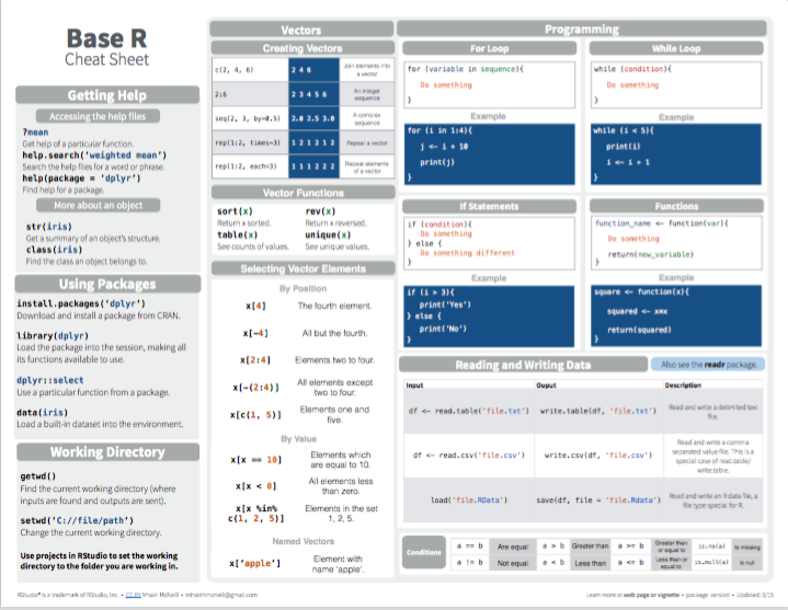
Figure 6.1: Base R summary from Posit cheatsheets.
For an overview of the map() functions of the purrr package, see the corresponding summary from Posit cheatsheets:
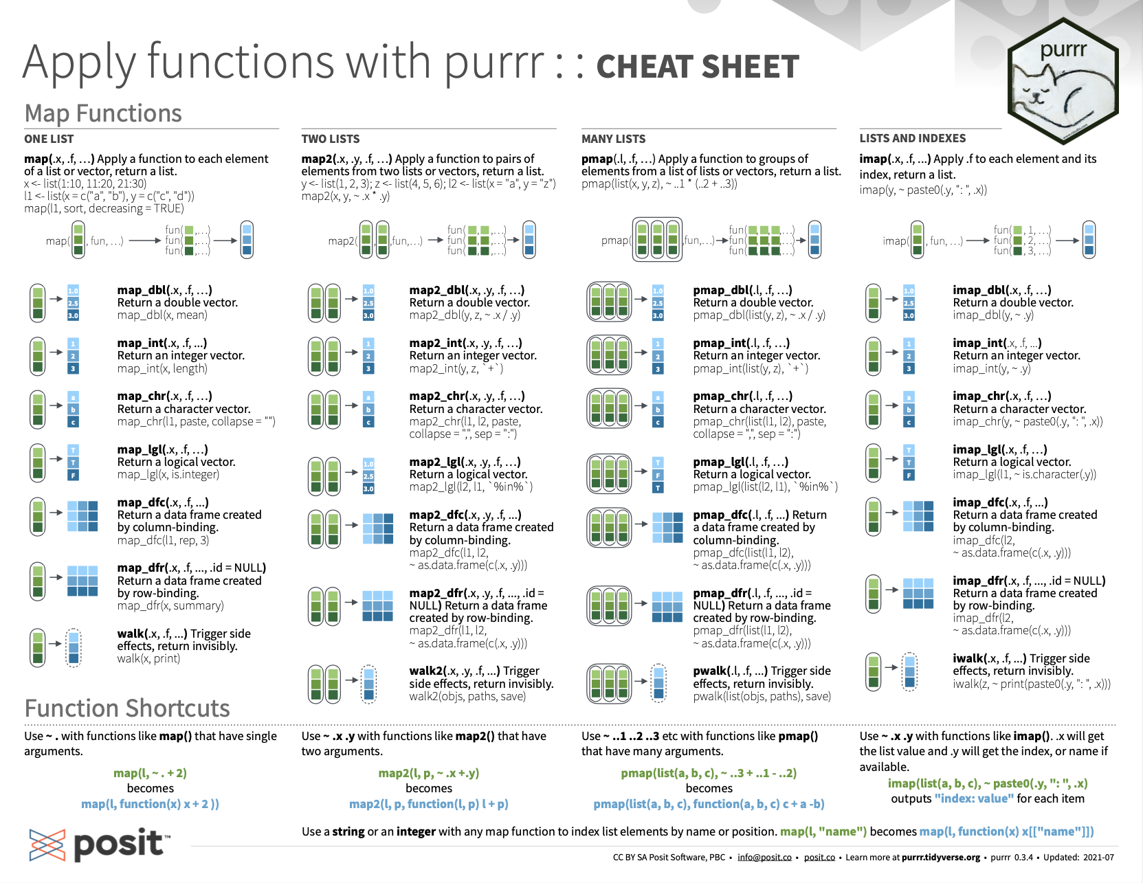
Figure 6.2: Overview of the map() functions of purrr from Posit cheatsheets.
For additional resources in iteration, see Section 12.7 of the ds4psy book (Neth, 2025a).
6.4.3 Preview
This chapter concludes Part 2 of this book and our introduction to programming basics in R. The upcoming Part 3 addresses various aspects of visualizing data. The introductory Chapter 7 reflects on the purposes, elements, and evaluation of visualizations. Chapters 8 and 9 will then enable us to create visualizations (using base R functions or the ggplot2 package). Chapter 10 deals with the representation and manipulation of colors and color palettes.
6.5 Exercises
Here are four exercises from 12.5: Exercises of the ds4psy book (Neth, 2025a):
6.5.5 Explicit vs. implicit iteration
Explain the difference between explicit and implicit iteration in your own words. The answer the following questions (e.g., by thinking of examples):
Which types of loops can immediately be replaced by implicit iteration?
Which aspects or types of loops can not be replaced by implicit iteration?
6.5.6 Applying a divisor checking function
- Re-solve Part 1. of Exercise 2 by creating a
is_divisor(x, N)verification function (that evaluates toTRUEiffxis a divisor ofN) and use a function from theapply()family of functions to applyis_divisor()to a data structure that contains the natural numbers from 1 to 1000.
Beware: Is there a simpler solution to achieve the same result in R?
6.5.7 Bonus exercise: Explaining mapping functions
As this exercise involves advanced mapping functions, it is optional, but still worth trying.
- Predict, evaluate, and explain the results of the following expressions (which are examples copied the documentations of the corresponding functions):
# sapply(): ----
i39 <- sapply(3:9, seq) # data: list of vectors
sapply(i39, fivenum)

# mapply(): ----
mapply(rep, 1:4, 4:1)
mapply(rep, times = 1:4, MoreArgs = list(x = 42))

# tapply(): ----
tibble::as_tibble(datasets::warpbreaks)  # data frame
tapply(warpbreaks$breaks, warpbreaks[,-1], sum)- Try to re-write the expressions of 1. with purrr mapping functions.
This concludes our exercises on iteration by creating loops and applying functions.