10 Using colors

Every perception of colour is an illusion…
We do not see colors as they really are.
In our perception they alter one another.

Josef Albers, Wikiquote

The statement that “art is not an object” has been attributed to many different artists and authors, and is typically followed by an alternative attempt to define art (i.e., as an experience, a way of looking, etc.). The statement that “Art is not an object but experience” is often attributed to Josef Albers (1968, Wikiquote).²³ In his abstract series of paintings Homage to the Square, Albers contrasted a reduction to a formal minimum with a rich spectrum of colors to evoke both intellectual and emotional experiences.

The interplay between objective and subjective aspects of art is particularly clear in the perception of color. Rather than existing as passive objects in the world, colors are often described as attributes of objects and must be seen by a viewer to be perceived. As the experience of color requires an interaction between an object and a perceiving organism, the properties of both (e.g., light and surface structures, receptors, and interpretations) play crucial roles for the perception of color.

The active and interactive nature of color has not only inspired artists and designers. Beyond exploring the interactive and ephemeral nature of color in works of art, the systematic study of color has fascinated thinkers and scientists for centuries. Not only can a few blotches of paint on a canvass (or black letters on white paper) evoke all kinds of emotional experiences, but combinations of colors can give rise to an entire spectrum of biases, distortions, and illusions.

When moving beyond describing, arranging and classifying colors, grasping their nature requires a theoretical and practical understanding that involves many disciplines (including arts, humanities, and natural sciences).

The inter-disciplinary appeal and relevance of color concepts make color a grateful topic for studying data science. For most people, colors are perceptually obvious, but their underlying representation remains hidden and obscure. This allows to reflect some non-trivial details of alternative representations and observe the effects of changes in parameters in an intuitive and often surprising fashion. Additionally, the preceding chapters have shown that we need color to make more informative and pleasing visualizations. Hence, getting color-savvy will make us not only more knowledgeable, but also more effective designers.

Computer and data scientists aim to capture color descriptions and perceptual experiences in abstract representations and validate their conceptual insights by formal models. In the case of color, this results in systems that allow to measure and quantify visual notions like brightness, hue, or temperature. But as we will see, the theoretic arsenal of color theory will ultimately still depend on experience — both literally (as color only exist in the mind of the beholder) and practically (as good color design requires a lot of experience).

Preparation

Recommended background readings for this chapter include:

• Appendix D: Using colors in R of the ds4psy book (Neth, 2023a)

Preflections

• What are colors? How do we experience them?

• How many colors are there? Which of them do we know?

• How do we describe or refer to colors? Can we see colors for which we lack names?

• How can we define and create a particular color?

• When and why do we use color (e.g., in texts or visualizations)?

10.1 Introduction

Colors are an important aspect of visualizations, but also of our life in general. Given that artists, designers and psychologists are attributing all kinds of effects to colors, it is not surprising that color is a big topic in scientific and business contexts.

From a theoretical viewpoint, color is an ideal topic for teaching data science. Although it is clear that the bright and shiny surfaces of our digital screens must somehow be encoded in bits and bytes, most people have no idea how this is achieved. Even when learning more about the ways of representing color information, it remains fascinating how different systems can express the same color. Thus, colors do not only brighten up our lives, but issues of color representation raise puzzling questions regarding identity and similarity.

10.1.1 Representing color

Answering the question What are colors? is difficult. Although we habitually see and use colors (e.g., when reading a text or viewing a screen), it is not so clear whether they actually exist in the world or only in our minds. And while most of us have pretty clear color preferences, it is a mystery how these have been developed and are being shaped by our surroundings.

When reflecting on any representation, we first need to distinguish between its meaning and its description(s). Although making a precise distinction is philosophically challenging, the word meaning aims to capture the essential or substantial properties of a construct or thing, whereas the term description implies that there are alternative ways to relate or refer to it. For instance, the number \(1\) is defined within a mathematical system and as such endowed with certain properties (e.g., relations to other numbers). However, the same number can be called “one”, “eins”, or “uno” and written as \(\alpha\), \(i\) or \(|\), without these changes in language or notation affecting its meaning.

When considering the representation of color, we can distinguish three different levels:

• Physical properties: Wave-length of light, properties of sensors (e.g., in cameras or eyes).
• Perceptual properties: Visual appearance (Is some color hue more red or green?) vs. psychological aspects (happy or sad mood?)
• Descriptions: Details of some representational system (e.g., verbal names or values in some measurement system)

Equipped with these distinctions, we can ask: What constitutes similarity in colors? More precisely, in which respect are colors different or similar? Again, answering the question is more difficult than it first seems. Here are some motivating examples:

• Are the colors "black" and "beige" similar because they both have 5-letter names beginning with the letter “b”?

• Colors with similar appearance, but different names:

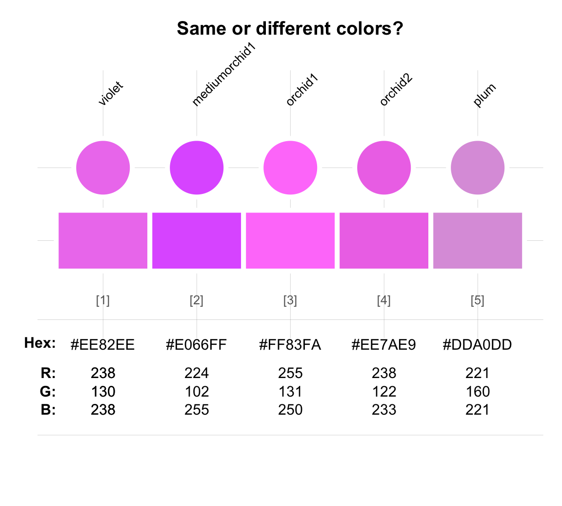
• Colors with different appearance, but similar names and values:

Any statement of identity or similarity requires an additional specification of the dimension or metric that is being used to measure similarity: In what respect are two entities identical or similar? This demystifies the apparent problems when two perceptually similar colors have different descriptions, or when two distinct colors have similar descriptions.

Psychological and semantic considerations

When designing colors or color palettes: Which colors go or fit together? Depends on intended uses, many more subtle factors, and heavily on the experience and expectations of the viewer. (Consider clothing, flags, and the logos of institutions or teams.)

10.1.2 Colors for the color-blind

Learning about colors enables us to design more effective and more pleasing colors and color schemes. However, knowing more about colors also renders us more sensitive to alternative forms of color vision. As large proportions of people see colors differently, we must not take a particular form of color perception for granted.

Our retina contains so-called rod and cone receptors. Whereas rod cells detect the intensity of light, cone cells are responsible for color vision. Most humans have three types of cones to take care of the different wavelengths that compose visible light and are thus capable of detecting a relatively wide spectrum of color. This most typical condition is called trichromia and most color schemes are designed by assuming this norm.

Some humans, however, — as much as 8% of the male population in many parts of the world — have inherited a missing or damaged cone, which prevents them from perceiving some colors. That condition is called dichromia, or coloquially referred to as “color blindness”. Depending on what cones or rods are damaged or missing, color blindness comes in many forms (e.g., selective impairments in protanopia, deuteranopia and tritanopia vs. total impairment in achromatopsia). While the precise perceptual effects vary by condition, their psychological consequences resemble each other: An affected person gets disturbed and confused when colors lack sufficient contrast or fall into one of their blind spots.

Choosing good colors is a difficult task when designing for “normal” vision, but designing for color blind users is more challenging. As with other so-called “impairments”, we can address and beat them on multiple fronts: Rather than accepting suboptimal conditions, we can aim to scaffold or overcome them by environmental changes. Due to their flexibility, computers are great tools for providing such support. Importantly, designing more effective interfaces requires being aware of and knowledgeable about color definitions and perception.

As a general rule, good graphic design should avoid the exclusive use of color coding to express information. When creating a graph, simply ask yourself whether all of it would still make sense when being viewed in black and white. Providing redundant codings not only helps the color blind, but also aids the comprehension of normally sighted people by providing them with multiple cues.

Finally, the topic of color raises many philosophical quandries: Do ripe cherries, strawberries and tomatos share some surface property that we perceive as being red? When looking at a brain scan, can we detect someone dreaming of a pink rabbit? If my red looks green to you, can we still talk about colors? In slightly more technical terms, we can ask:

• Are colors physical properties of objects or are they relational properties that require someone perceiving it?

• Can the experience of color vision be reduced to patterns in neuronal signals?

• What are the consequences if someone’s color perception was re-wired partially or completely?

For details, see Maund, B. (2022), Color, The Stanford Encyclopedia of Philosophy.

Beyond theoretical puzzles, the issue of color raises many practical questions:

• How can we define and use colors and color palettes?

• How can we find fitting colors and color palettes when creating documents and visualizations?

10.1.3 Contents

10.1.4 Data and tools

In this chapter, we study the named colors of and different ways to define color in base R. For manipulating color palettes and solving color-related tasks, we will use the unikn package, but less for its colors than for its color-related functions that make it easy to view colors, create new color palettes, as well as search for color names or for similar colors.

10.2 Essentials

The following sections cover three topics:

• Defining colors: Representing and classifying colors in R (see Section 10.2.1)
• Creating and using color palettes (see Section 10.2.2)
• Working with colors in R: Color-related tasks and corresponding recipes (see Section 10.2.3)

10.2.1 Defining colors in R

Colors can be represented in many different ways. More specifically, there are many alternative ways to analyze or synthesize colors, and the most appropriate representational way depends on the specific context of a particular use case (see Wikipedia: Color model for an introduction).

In R, the grDevices package (included in any default installation) provides colors and color-related functions. Although R supports many color models (including HCL, HSV, Lab, Luv, and RGB variants), the three most common ways of expressing colors in R are:

1. by R color name: R includes 657 named colors, whose names are provided (as a character vector) by evaluating the colors() function of grDevices.

2. by RGB values: Every color (or hue) is expressed by a triple of numeric values on three dimensions that denote the additive primary colors (red, green, blue). The range of values is either expressed on a scale from 0 to 1, or — more typically — on a scale from 0 to 255 (i.e., on an 8 bit scale allowing for \(2^8 = 256\) different values).

3. by HEX values: Every color (or hue) is expressed by a character string (with the prefix #), followed by a triple of hexadecimal values (each ranging from 00 to FF) that correspond to the triple of decimal RGB values (in range from 0 to 255).

Importantly, the same color (or hue) can be denoted by its name, its RGB values, and its HEX values. Thus, the three different systems (i.e., color name, RGB values, or HEX values) can be alternative representations of the same object. However, just as the properties of an alphabet or numeral notation system constraints the words or numbers that can be expressed by it, the universe of possible colors is limited by their representation. For instance, whereas the RGB and HEX color systems usually distinguish between more than 16 million (i.e., \((2^8)^3 = 256^3 = 16.777.216\)) possible colors, only a limited number of them are named. Similarly, when multiple names refer to the same triple of RGB or HEX values, they denote the same color.²⁴

An example helps clarifying these abstract terms. When viewing an existing color or color palette with the seecol() function of unikn, the name, HEX and RGB values of the individual colors are being shown. For instance, Figure 10.1 shows some colors of the Max Planck Society:

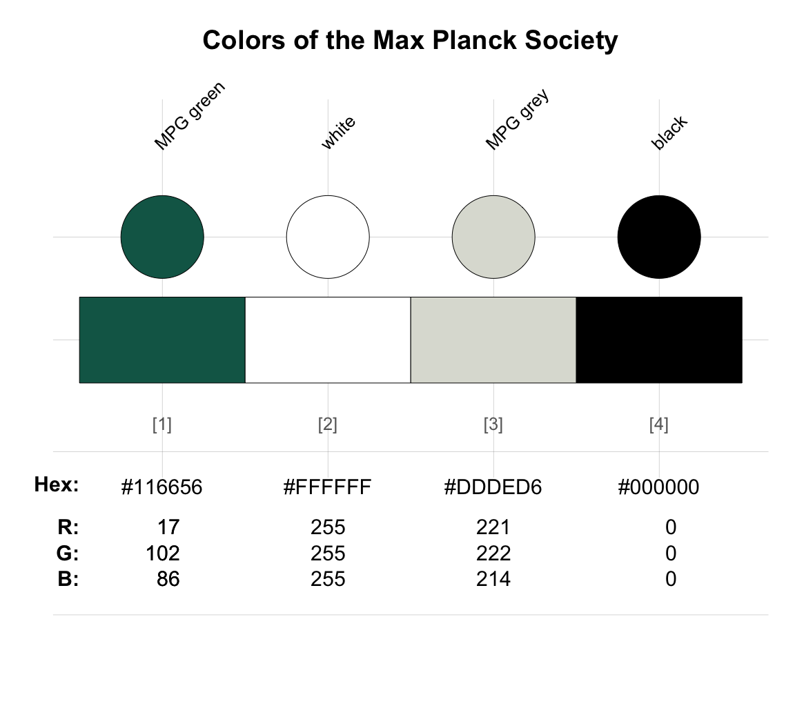
Figure 10.1: Viewing colors with seecol() of the unikn package shows their names, HEX, and RGB values.

Each color shown here is described by a name (e.g., “black”), a triple of HEX values (#000000), and a triple of RGB values (R: 0, G: 0, B: 0). These three representations provide alternative ways of describing and using the same color.

As the 6th and 3rd colors (“black” and “white”) are two of the 657 named colors of colors(), R will recognize them as colors when we type their name (as character objects "black" or "white") in a context that expects color inputs. However, other colors shown in Figure 10.1 have either been defined by the Max Planck Society (e.g., "MPG green") or were created by mixing other colors (e.g., "MPG green 50%" is a mix of "MPG green" and "white"). As custom colors are usually not pre-defined colors of R (i.e., not contained in colors()), we must learn to define them as colors objects before we can use and manipulate them in R.

Named colors in R

The simplest system of colors in R is not very systematic, but can be very intuitive to use — provided that the user is familiar with the color names. The grDevices package defines two basic functions that provide basic color support:

1. palette() provides 3 elementary colors (as a categorical color palette):

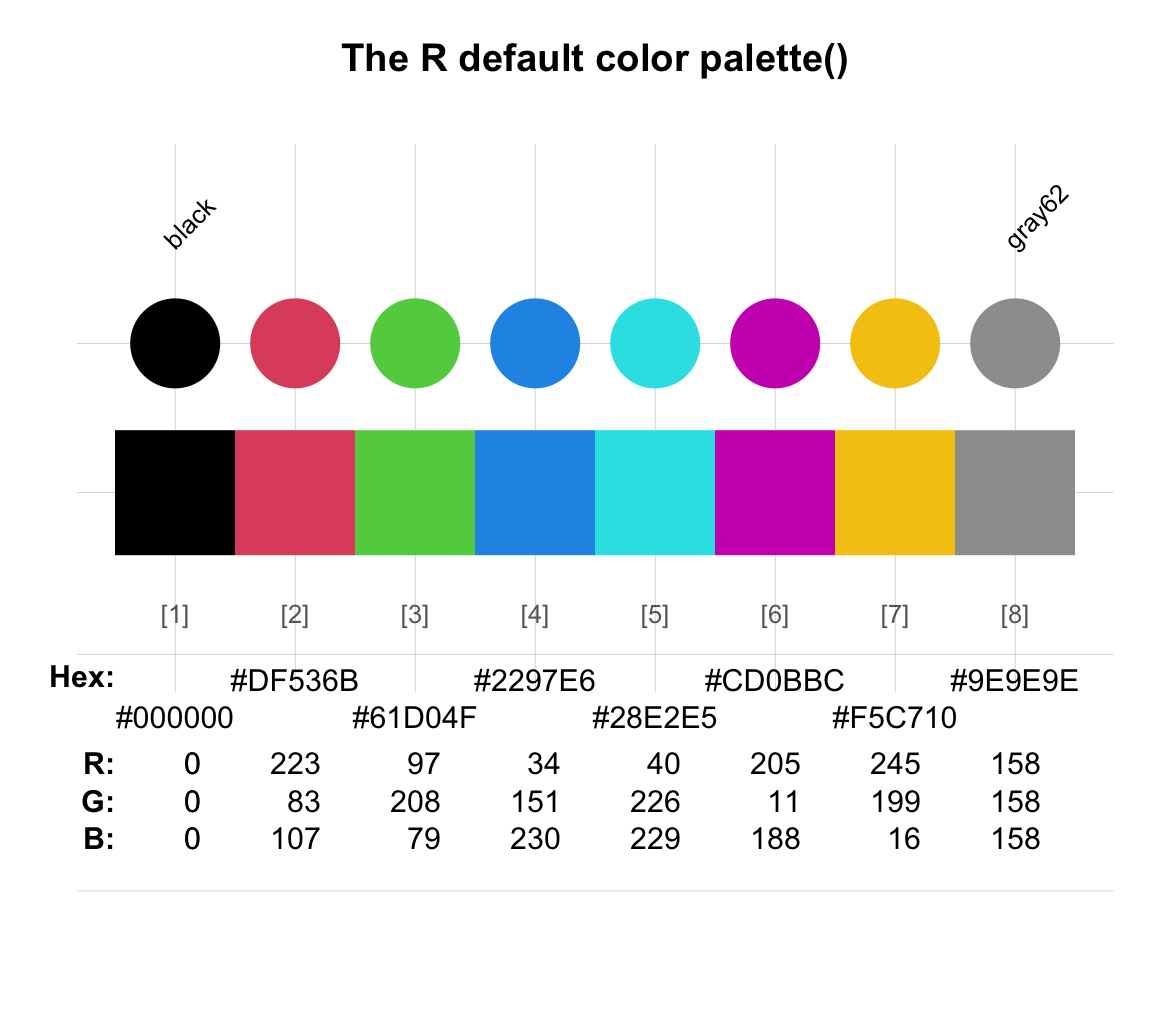
Figure 10.2: The default color palette() of R (using R version 4.3.2 (2023-10-31)).

Many R plotting functions allow specifying colors by a numeric index (e.g., col = 2), rather than a name. When choosing a color by a number \(i\), R internally provides the \(i\)-th element of the color vector palette():

palette() # vector of R default color names
#> [1] "black"   "#DF536B" "#61D04F" "#2297E6" "#28E2E5" "#CD0BBC" "#F5C710"
#> [8] "gray62"
palette()[c(1, 2, 7)]  # 3 named colors
#> [1] "black"   "#DF536B" "#F5C710"

2. colors() provides 657 named colors that have descriptive names, some of which have multiple shades.

Figure 10.3 shows a random sample of 200 colors (from all 657 colors, but excluding its 224 shades of grey and gray):

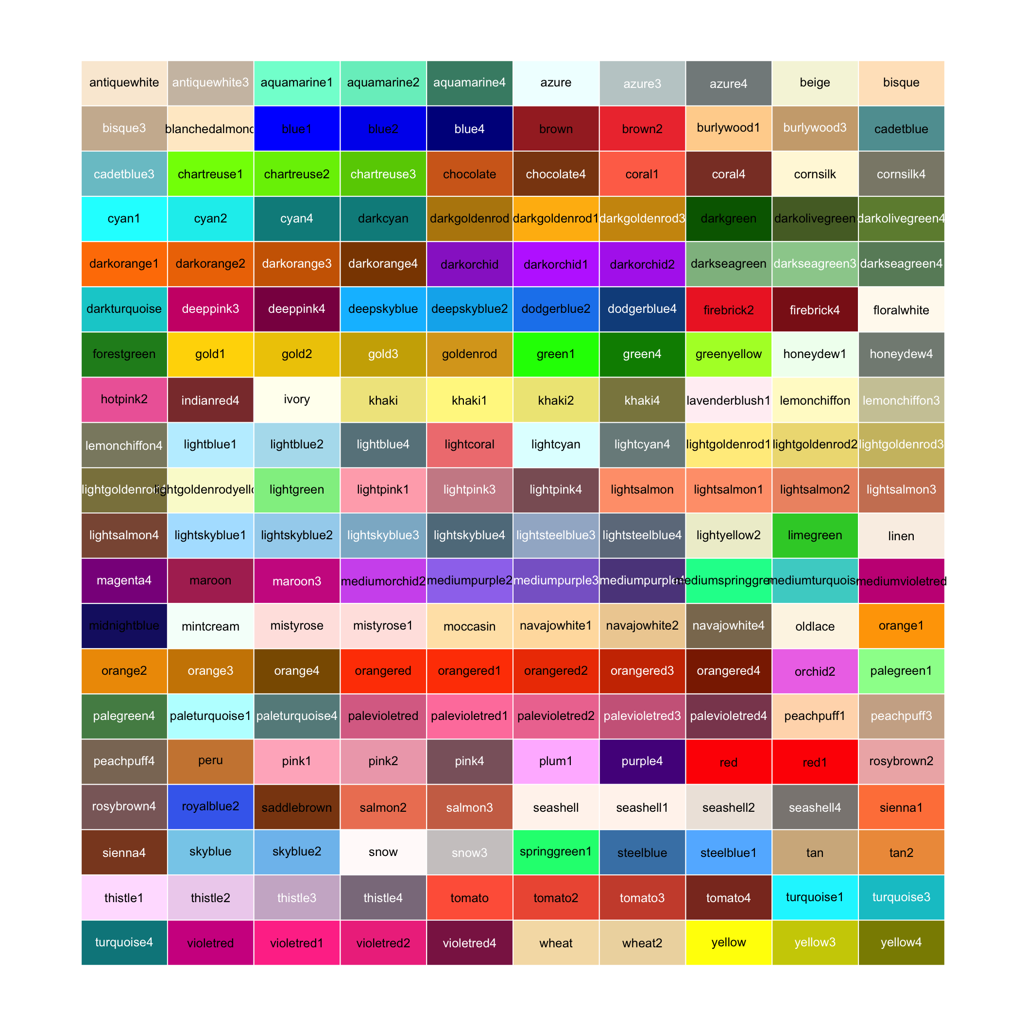
Figure 10.3: 200 random (non-gray) colors (from colors()) and their names in R.

Figure 10.3 shows that there is no shortage of vibrant colors in R. Despite considerable variability, we can detect two quasi-systematic aspects in their variety:

First, their names aim to provide verbal descriptions of the corresponding color. Although many names are somewhat exotic (e.g., "blanchedalmon" or "mistyrose"), they also provide descriptive elements: So-called dark colors are more intense than their light or pale varieties.
Thus, the R color names correspond to our conceptual understanding of colors, even when our world knowledge relates hues to typical objects (e.g., colors with sky are bluish, hues of salmon appear fishy, variants of lemon are yellowish, and snow is some greyish white).

Second, many colors have several numeric variants (e.g., "gold1", "gold2", \(\ldots\) gold\(n\), with \(n = 4\)). Here, higher numbers correspond to darker versions of a color.

Together, these two systematic elements enable an informed choice of colors. We can perform a quick quizz on ourselves: What does the R color named "steelblue" look like? We have a pretty clear idea what to expect for blue (as the color of eyes, water, or the sky, etc.). Perhaps the qualifier steel suggest a colder and greyer version?

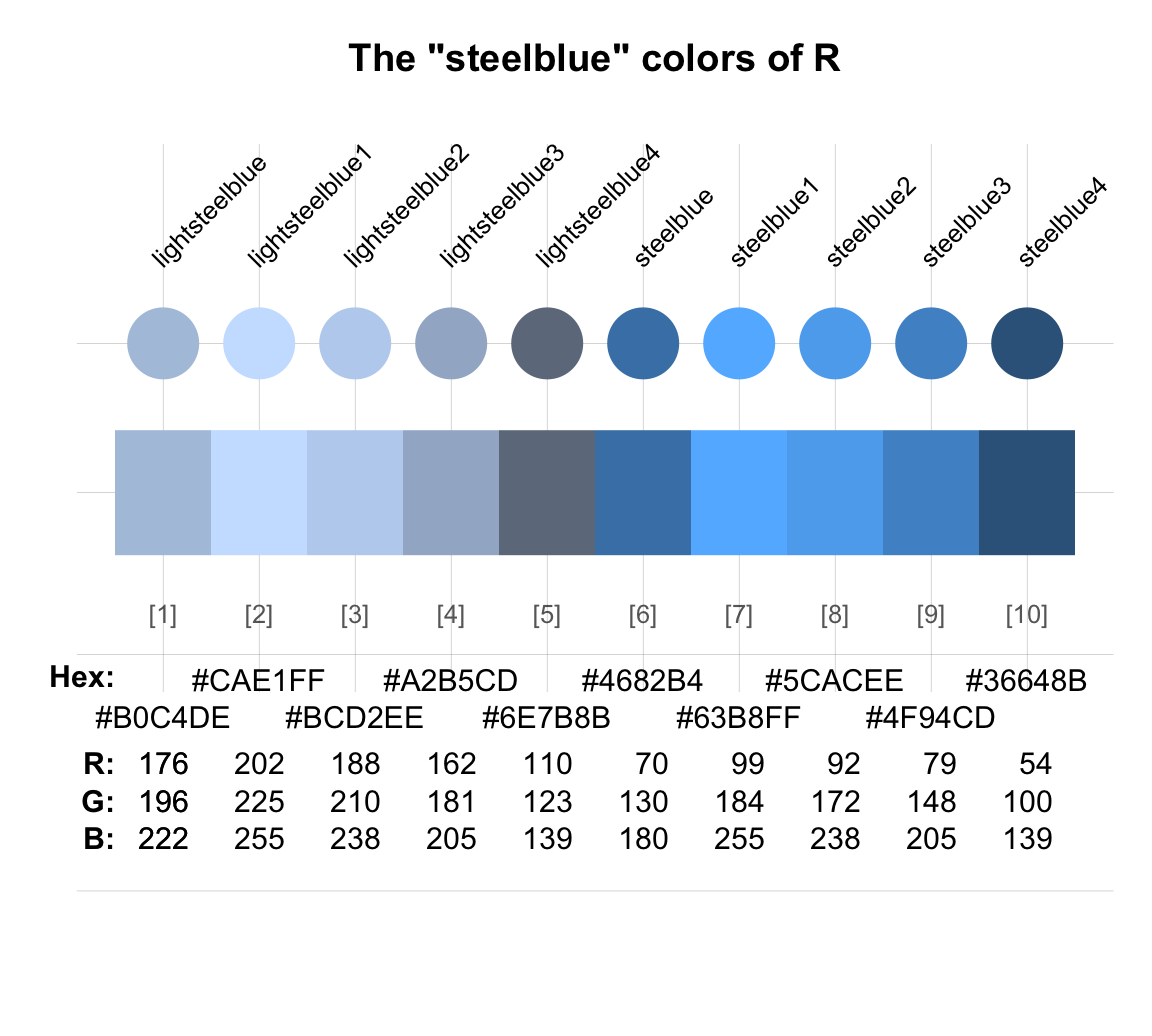
Figure 10.4: R colors() with ‘steelblue’ in their names.

Figure 10.4 verifies that the 10 "steelblue" colors from colors() belong to a family that mixes blue and grey color hues. As expected, the “light” variants tend to be brighter than the regular variants. Of both "lightsteelbue" and "steelblue", there exist four enumerated variants (with suffixes 1 to 4) that denote increasingly darker shades. Interestingly, neither "lightsteelbue" nor "steelblue" correspond exactly to one of their enumerated variants (see their unique HEX and RGB values).

Overall, using the 3 colors of palette() or the 657 named colors of colors() offers both advantages and disadvantages. The key advantage is that they are readily available (as the grDevices package comes with an installation of R) and that they are quite easy and intuitive to use. A limitation is that verbal color labels are often imprecise and thus the color names may not correspond to our expectations. For instance, the color "maroon" is typically seen as brownish-red, but R renders it as purple-violet. Similarly, some shades of "brown" appear indistinguishable from varieties of pink or red.²⁵

The main limitation of using named colors in R is that they make it hard to create good color palettes Interestingly, this difficulty is the price for the ease with which we access the colors. Descriptive verbal labels allow us to easily select different colors, but provide no way to identify and combine matching colors into color palettes.

Unfortunately, choosing and combining colors from the list of colors() resembles a lottery: We can get lucky, but in most cases the outcome will be disappointing. A more promising approach is to use color palettes that were designed for specific purposes or to create dedicated color palettes that follow common principles and thus are more likely to fit together.

In the following, we will first learn about some properties of formal color systems. Beyond making us more color-wise, this will enable us to define and design our own colors and color palettes. Afterwards, we will see that many R packages provide dedicated color palettes that have been designed for a variety of purposes.

Formal color systems

Using a formal color system enables a more principled and systematic approach to colors. The price of formal systems is that they usually involve some terminology and notational conventions. For instance, many systems distinguish between two aspects of an individual color:

• The hue of a color describes its primary components (e.g., mostly red, green, or blue) but often includes aspects of its appearance or impression that may depend on context or recipients (e.g., bright/dark shades, cold/warm temperature). Depending on the color system, hue can be specified as a set of values on different dimensions or as a single value on some scale.

• The opacity or transparency of a color regulates how the color interacts when overlapping with other colors. We typically vary this property on a continuous scale (usually by providing an alpha value in the range from 0 to 1).

The fact that hue and opacity are different concepts, but visually influence each other (as a semi-transparent color appears as mixed with the hue of the background) illustrates the need for clear definitions.

Many systems have additional terms or parameters for specifying the intensity of non-transparent colors. Their specific terms depend on the particular color system we want to use.
For instance, the HCL color system defines colors by their hue, chroma, and luminance values, whereas the HSV color system specifies them by hue, saturation, and value.

As we cannot cover all systems here, we will focus on the most common RGB color system and a notational variation of it that expresses the decimal RGB values in hexadecimal (HEX) values.

Using RGB values

The RGB color system is based on three primary colors (i.e., RGB is an acronym for _R_ed, _G_reen, and _B_lue). It is based on the insight that these three primary colors can be mixed in an additive fashion to create a rich spectrum of secondary colors.

A physical model of the RGB system is provided by superimposing three beams of light. When doing so, the wavelengths of the component colors add up to make up the mixed colors of overlapping regions. Beyond providing an abstract model for analyzing and defining colors, the RGB color system is widely used in electronic devices (e.g., in CRTs, or LCD and OLED displays), non-digital photography, and its theory is related to human color perception (see Wikipedia: RGB color model for details).

From a notational viewpoint, the RGB system defines a color by a triple of numeric values that denote its intensity on each of the three primary color channels or dimensions (i.e., Red, Green, and Blue, respectively). The numeric values typically range from a minimum of 0 to a maximum of 1 or — when honoring the traditional 8-bit representation — from 0 to 255 (i.e., each channel allows for \(2^8 = 256\) different values).

Technically, using the rgb() function of the grDevices package allows defining RGB colors in R and enables a systematic approach for understanding the definition of colors in the RGB system. For instance, we can ask:

• What are the most extreme values within the system? Which colors are defined when setting all three channels to the minimum or maximum value?

We can use the rgb() function of the grDevices package to define two color objects (named c_000 and c_111) with extreme values in the range from 0 to 1:

# A: Black vs. white: Maximize contrast (on all 3 dimensions): ------ 
c_000 <- rgb(red = 0, green = 0, blue = 0, alpha = NULL, names = "Color 000", maxColorValue = 1)
c_111 <- rgb(red = 1, green = 1, blue = 1, alpha = NULL, names = "Color 111", maxColorValue = 1)

Here is how the corresponding colors (of our objects c_000 and c_111) look:

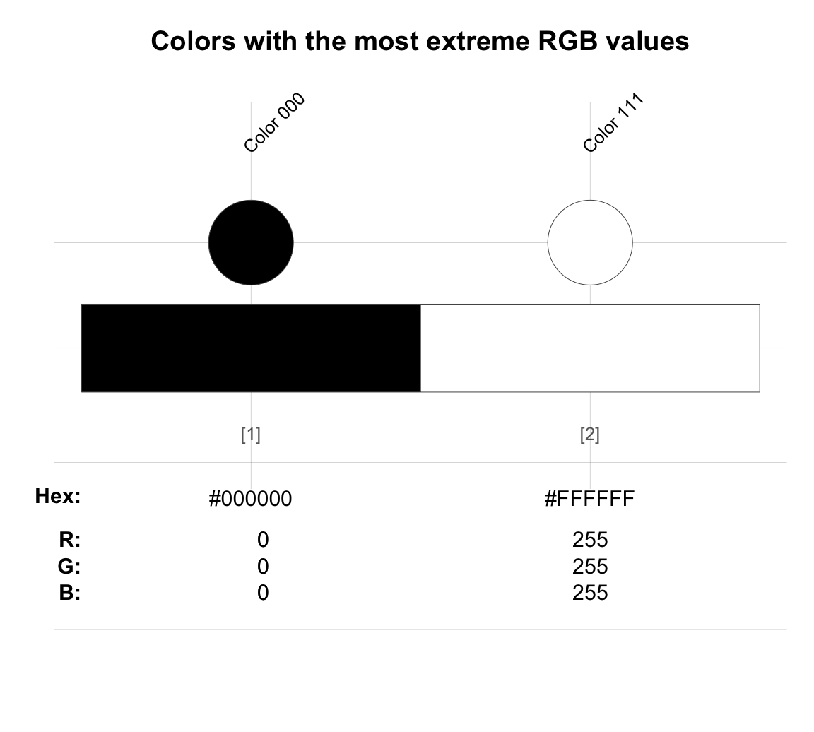
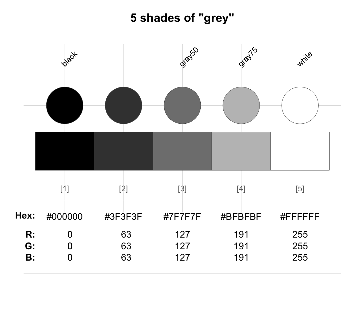
Thus, we can see that — in the RGB color system — the absence of any color values (i.e., the triplet \((0, 0, 0)\)) denotes the color "black" and a maximum intensity of all primary colors (i.e., the triplet \((255, 255, 255)\)) denotes the color "white". Perhaps not surprisingly, a balanced triplet of intermediate color values on all three dimensions denote different shades of "grey":

Another good question with an instructive answer is:

• Which colors result from maximizing RGB values on exactly one dimension (while minimizing the others)?

Again, we use the rgb() function to define corresponding color objects (named c_100, c_010 and c_001):

c_100 <- rgb(red = 1, green = 0, blue = 0, alpha = NULL, names = "Color 100", maxColorValue = 1)
c_010 <- rgb(red = 0, green = 1, blue = 0, alpha = NULL, names = "Color 010", maxColorValue = 1)
c_001 <- rgb(red = 0, green = 0, blue = 1, alpha = NULL, names = "Color 001", maxColorValue = 1)

Figure 10.5 combines all five color objects:

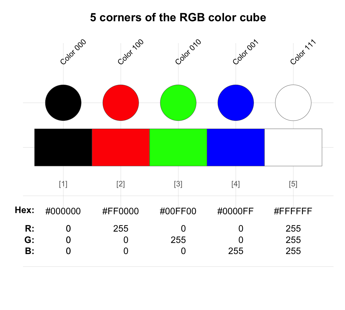
Figure 10.5: Basic color values in the RGB color system: A numeric value represents the intensity of each each primary color. On each channel, lower values correspond to darker colors, higher values correspond to brighter colors.

Figure 10.5 shows the three primary colors embedded within the two most extreme colors. More specifically, when expressing the RGB values on a scale from 0 to 255, the three primary colors (that maximize exactly one color channel) appear as red \((255, 0, 0)\), green \((0, 255, 0)\), and blue \((0, 0, 255)\).

Geometrically, each triplet of RGB values represents a point in a 3-dimensional color space. When the orthogonal dimensions denote the intensity of each primary color (e.g., on a scale ranging from 0 to 1), the extreme corners of the resulting cube denote black \((0, 0, 0)\) and white \((1, 1, 1)\), with three other corners denoting the primary colors red \((1, 0, 0)\), green \((0, 1, 0)\), and blue \((0, 0, 1)\) (see the 3D-visualization at Wikipedia: RGB color model: Geometric representation).

The fact that black results from the absence of colors (e.g., RGB values of \((0, 0, 0)\)) and white results from the addition or super-imposition of all three primary colors (e.g., RGB values of \((1, 1, 1)\)) is an initially counter-intuitive aspect of the RGB color system. More generally, lower values on a component or channel correspond to darker colors and higher values on a component or channel correspond to brighter colors. Thus, we can sometimes estimate the appearance of a mixed color by interpreting its RGB values. For instance, a color with a high value on the R channel and low values on the G and B channels is likely to appear as some shade of red.

Although the results of more complex combinations of color values are often difficult predict, it is obvious that the standard RGB system can define and distinguish between more than 16 million (i.e., \((2^8)^3 = 256^3 = 16.777.216\)) possible colors. As an example, the following visualization shows the appearance, color name, RGB and HEX values of four colors that was defined as a vector of named colors my_cols:

my_cols <- c("firebrick", "olivedrab3", "orange", "steelblue")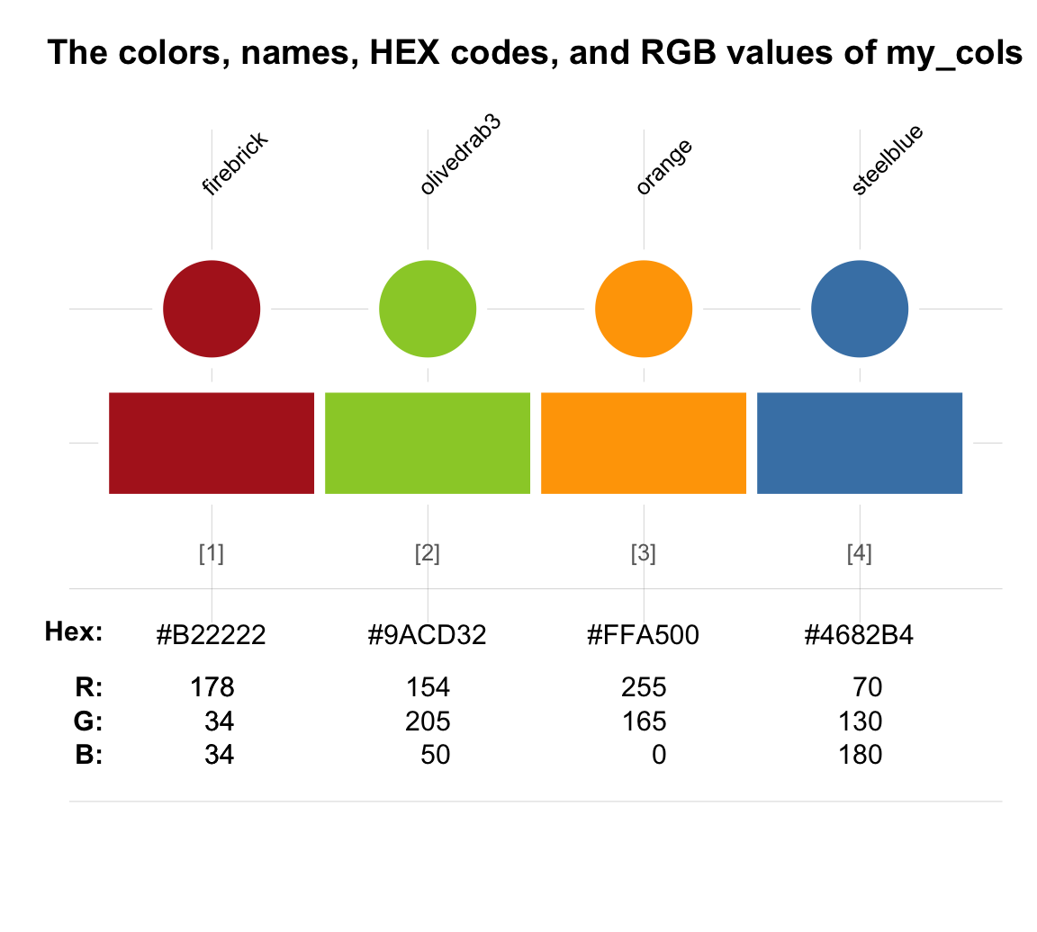

A summary on the RGB color model:

• The additive RGB color model contains channels for each of three primary colors: Red, Green, and Blue.
• Each color channel expresses the corresponding intensity on a standard range (e.g., from 0 to 255, i.e., 8-bit)
• Complete absence of colors yields "black", a maximum presence of all colors yields "white".
• A triple of identical values on all dimensions define 256 shades of "grey".
• Over 16 million other colors can be expressed as combinations of RGB values (i.e., an additive mix of the three primary colors).

Using HEX values

A good question to ask at this point is:

• What do we obtain when we evaluate our custom color objects?

We can easily find this out by defining a new color object with rgb() and then evaluating it. For instance, Figure 10.1 (above) showed that the color "MPG green" (or mpg_pal[1]) corresponds to the triple of RGB value (17, 102, 86):

# From RGB values:
mpg_green <- rgb(17, 102, 86, names = "MPG green", maxColorValue = 255)
mpg_green  # evaluates to corresponding HEX values:
#> MPG green 
#> "#116656"

# Contrast for a named color:
"firebrick"  # evaluates to a character object, rather than to HEX values: 
#> [1] "firebrick"

This shows that, when evaluating a color object created by rgb(), R returns a character sequence of the form "#RRGGBB". (By contrast, evaluating a named R color still yields the name of the color, as a character object.) In the character string with the #-prefix, the symbol sequence RRGGBB expresses the three RGB values (for the Red, Green, and Blue channel, respectively) in hexadecimal (HEX) notation (i.e., in the base-16 notation for the range of values from 0 to 255). In HEX notation, the ten numeral symbols (i.e., the digits from 0 to 9) or the decimal system are extended by the first six letters of the alphabet (i.e., A to F) to turn our usual base-10 notation into an analogous place-value notation with a base of 16. Thus, the HEX value of "#116656" is merely a more compact way of expressing

• Red: \(1 \cdot 16 + 1 = 17\)
• Green: \(6 \cdot 16 + 6 = 102\)
• Blue: \(5 \cdot 16 + 6 = 86\)

Defining colors from their HEX values

The equivalence of the RGB and HEX notations can be demonstrated by defining the same colors a second time, but now directly specifying their HEX values (shown above):

# Redefining basic RGB colors (as named HEX colors):
rgb_cols_2 <- c("#000000", "#FF0000", "#00FF00", "#0000FF", "#FFFFFF")
names(rgb_cols_2) <- names(rgb_cols)

# Redefining a unikn color (as named HEX color):
mpg_green_2 <- "#116656"
names(mpg_green_2) <- names(mpg_green)

If those re-definitions really yield identical R objects, the following checks must evaluate to TRUE:

all.equal(rgb_cols, rgb_cols_2)
#> [1] TRUE
all.equal(mpg_green, mpg_green_2)
#> [1] TRUE

Thus, we can define colors from both their RGB or from their HEX values — and the two notations are really just two alternative ways of representing the same colors.

Decimal vs. hexadecimal notation

The HEX values of a color may look a bit cryptic, but are merely a convenient convention for expressing the RGB values. To understand their relation, we need to take a brief detour into the realm of numerical notation systems.

The HEX values of a color are translations of the RGB values (in decimal notation and a range from 0 to 255) into a hexadecimal numeral system. To read HEX values, we need to generalize the properties of our familar decimal (base-10) system to a hexadecimal (base-16) numeral notation system. Both our familiar Hindu-Arabic decimal system and the hexadecimal systems are positional number systems: The value of a numeral symbol depends not only on the symbol’s identity (e.g., \(2\)), but also on its position (e.g., the \(2\) in \(123\) means \(20\)).

The decimal notation system uses 10 different symbols (aka. digits or numerals) to represent the 10 distinct numeric values from \(0\) to \(9\) and a place-value notation to express numeric values beyond \(9\) as abbreviated polynomials. For instance, the three digit decimal notation \(123\) is actually an abbreviation for the numeric value of \(1 \cdot 10^2 + 2 \cdot 10^1 + 3 \cdot 10^0\). The fact that we typically are not even aware of this polynomial shows how familiarity with a representation can obscure its properties. But this familiarity is easily challenged when changing the base of the polynomial!

A hexadecimal notation system (HEX) uses the same 10 initial symbols, but extends their range by adding more symbols to express 16 distinct numeric values (i.e., the values from \(0\) to \(15\) are expressed by a single symbol). As the decimal system stops at a maximum value of \(9\), the hexademical system represents the decimal values \(10\) to \(15\) by the letters \(A\) to \(F\). Numeric values of \(16\) and beyond are expressed by using the same polynomial convention as in the decimal system. Thus, the two digit sequence \(10\) (in HEX notation) now represents a numeric value of \(16\) (in decimal notation), and the numeric value of the digit sequence \(123\) (in HEX notation) represents a value of \(1 \cdot 16^2 + 2 \cdot 16^1 + 3 \cdot 16^0 = 291\) (in decimal notation).

The following Table lists the first 20 symbols (or symbol combinations, for numeric values ranging from zero to nineteen) in both the decimal and HEX notation:

Symbol Nr.:	1	2	3	4	5	6	7	8	9	10	11	12	13	14	15	16	17	18	19	20
Value in decimal notation:	0	1	2	3	4	5	6	7	8	9	10	11	12	13	14	15	16	17	18	19
Value in HEX notation:	0	1	2	3	4	5	6	7	8	9	A	B	C	D	E	F	10	11	12	13

We can further explore the relation between the decimal and hexadecimal notation systems by the dec2base() and base2dec() functions of the ds4psy package:

library(ds4psy)

# Decimal to hexadecimal (base 16):
dec2base( 9, base = 16)
dec2base(10, base = 16)
dec2base(15, base = 16)
dec2base(16, base = 16)
dec2base(20, base = 16)

# Base 16 to decimal:
base2dec("10", base = 16)  # 16 x  1
base2dec("F0", base = 16)  # 16 * 15
base2dec("F9", base = 16)  # 16 * 15 +  9
base2dec("FF", base = 16)  # 16 * 15 + 15
base2dec("123", base = 16) # (1 * 16^2) + (2 * 16^1) + (3 * 16^0) 

# Comparing symbol lengths:
dec2base(1000000, base = 16)
dec2base(1000000000, base = 16)

Overall, the decimal and hexadecimal systems are very similar, but the former is much more familiar to us. When comparing both systems, we essentially see a trade-off of their basic alphabet size versus length of strings for expressing numeric values. More specifically, the HEX notation requires more elementary symbols than the decimal notation (16, rather than 10), but this allows it to express larger numeric values more compactly (e.g., a desimal value of \(1.000.000\) is expressed as \(F4240\)).

Practice

RGB and HEX values of named colors

Identify some colors with particularly outrageous R color names:

• How would you expect these colors to look?
• Use the demopal() or seecol() functions of the unikn package to visualize the colors.
• What are their RGB and HEX values?
• Do the colors look as you expected?

The additive RGB color model

Answer the following questions by running the following R commands:

1. What is the relation between the named R colors "red", "green", and "blue" and the RGB color model?

# Inspect colors (to view HEX and RGB values):
unikn::seecol(pal = c("red", "green", "blue"), 
              main = "The primary RGB colors")

2. What are the positions of the named R colors "cyan", "magenta", and "yellow" in the RGB color model?

# Inspect colors (to view HEX and RGB values):
unikn::seecol(pal = c("cyan", "magenta", "yellow"), 
              main = "The primary CMY colors")

3. The CMY color model is a subtractive color system that defines colors as reflected surface light, rather than as adding beams of light. It is used for mixing paints and dyes from three primary colors cyan, magenta, and yellow, whose combination at full intensity yields black (see Wikipedia: CMY color model for details). Use the seecol() function and your insights from 1. and 2. to answer the question:

• What is the relation between the primary colors of the RGB and the CMY color models?

Solution

The three primary RGB colors and the three primary CMY colors are located at 6 corners of a RGB (or CMY) color cube. More specifically, the primary colors of the (subtractive) CMY color model are the complements of the primary colors of the (additive) RGB color model (i.e., located at the opposite corner of a 3D-color cube). Thus,

• cyan is the absence of red at full intensity of green and blue;
• magenta is the absence of green at full intensity of red and blue;
• yellow is the absence of blue at full intensity of red and green.

Overall, the two extreme value combinations (black and white), three primary RGB colors (red, green and blue), and three primary CMY colors (cyan, magenta, and yellow) denote the eight corners of a 3-dimensional RGB (or CMY) color cube:

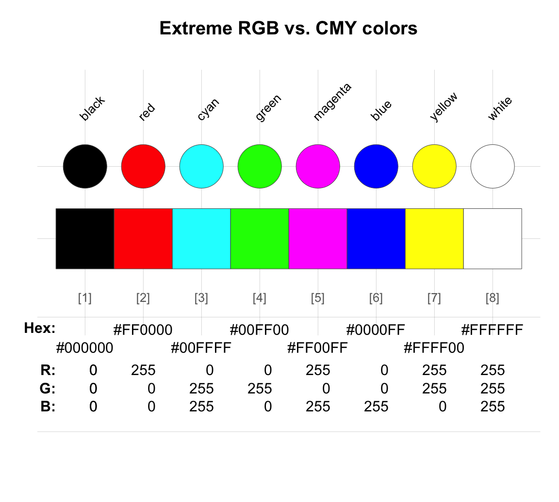
Figure 10.6: The 8 corners of a RGB / CMY color cube

Re-creating a named R color from RGB and HEX values

Pick an arbitrary name from the named R colors(), then

1. Re-define two new color objects from the color’s RGB and HEX values.

2. Demonstrate that all three R color objects yield the same color.

Solution

# 0. Pick a named color:
my_col_org <- "firebrick"

# Re-defining from RGB and HEX values: ----

# a. from RGB:
col_rgb <- col2rgb(my_col_org)  # find out RGB values
my_col_RGB  <- rgb(t(col_rgb), maxColorValue = 255)

# b. from HEX:
my_col_RGB  # evaluates to find out HEX values
my_col_HEX <- "#B22222"


# 2. Demonstrate equivalence: ---- 

# By inspecting the color objects:
seecol(c(my_col_org, my_col_RGB, my_col_HEX))

# By comparing underlying representations:
all.equal(col2rgb(my_col_org), col2rgb(my_col_RGB))
all.equal(col2rgb(my_col_org), col2rgb(my_col_HEX))

10.2.2 Creating and using color palettes

A color palette is an ordered sequences of colors, typically represented as a (named) vector or a data frame in R. A key characteristic of a useful color palette is that its colors must fit to each other. To the agony of many R users, simply picking a few colors from the range of named colors in colors() is unlikely to yield a good color palette. However, what would make a “fitting” or “good” palette depends on the visualization task at hand.

Three aspects to distinguish for a given color palette are:

1. its number of colors;
2. the relation of its colors to each other;
3. the relation of its colors to the current visualization goal/task.

Whereas these aspects 1 and 2 are internal features of a palette, aspect 3 concerns how suitable the palette is for a given task.

Types of color palettes

Which palette we use should always depend on the type of task that we are trying to solve.

• See D.2.2 The functions of color for different reasons for using color.

• See D.2.3 Types of color palettes for examples of different color palettes for different purposes. For instance, we can distinguish between:

  • categorical vs. continuous color palettes
  • bi-polar and divergent palettes
  • hybrid/ and paired color palettes

Using color palettes

The difficulty of finding matching colors is one reason why expert visual designers typically prefer using pre-defined color palettes. Another reason is to convey a uniform look or consistent image (e.g., of corporate identity).

Many dedicated R packages provide color palettes:

• See D.4 Using color packages of the ds4psy textbook (Neth, 2023a).

Creating new color palettes

When one of more colors have been defined, we may want to:

• Combine them into a color palette

• Extrapolate them into wider ranges

In principle, we could define color palettes as named vectors or as data frames. Here is a simple example for defining a new color palette with the newpal() function of the unikn package:

library(unikn)

# Defining a new color palette:
de_pal <- newpal(col = c("black", "red3", "gold"), 
                 names = c("really dark", "my red", "my gold"), 
                 as_df = FALSE)
# de_pal

# Inspecting new palette:
seecol(de_pal, main = "A new 'de_pal' color palette")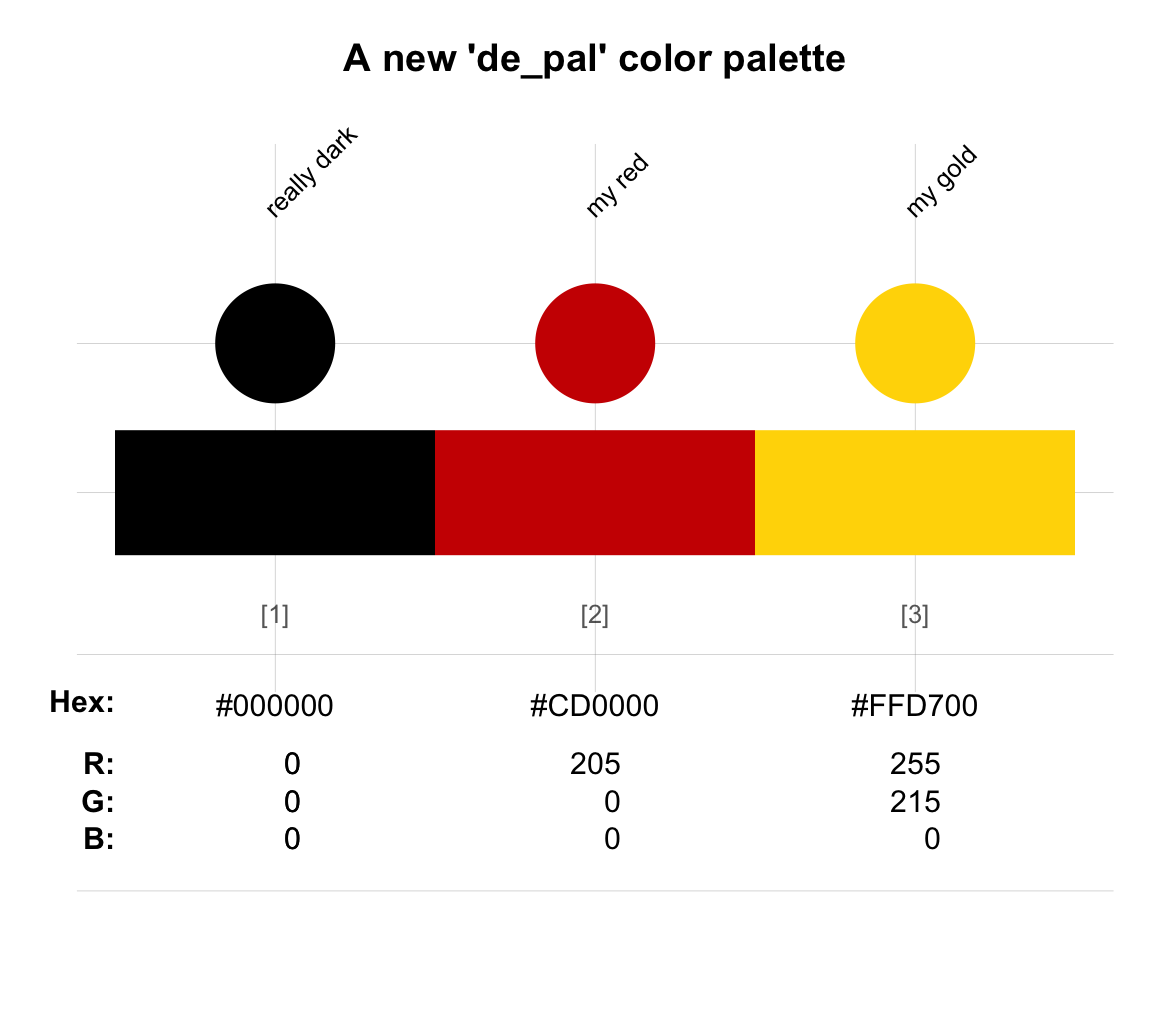

# An example plot:
demopal(de_pal, type = "mosaic")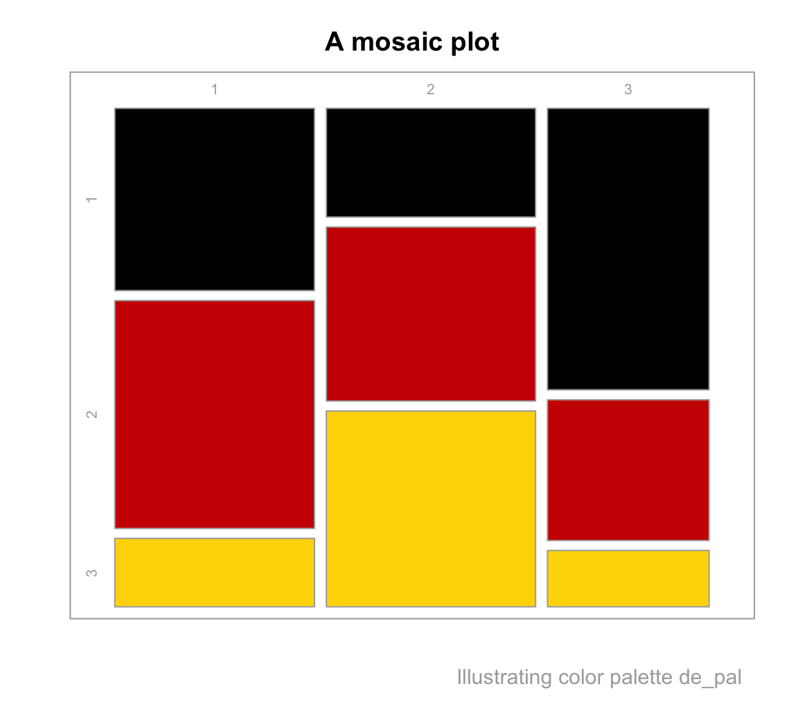

Extrapolating from a given color palette:

seecol(usecol(de_pal, n = 5), main = "Extrapolating a color palette")

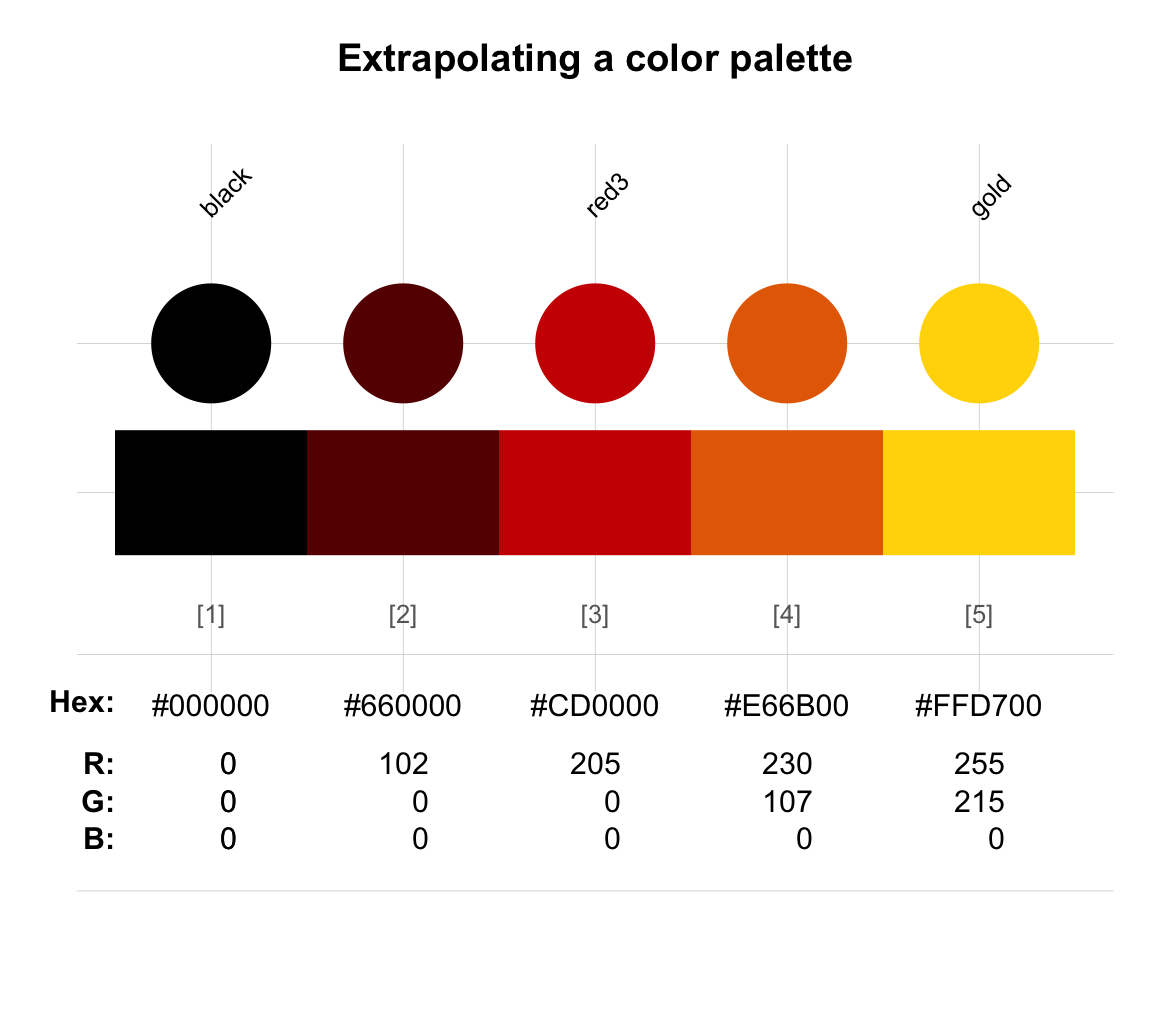
Providing an additional color and an argument n to the usecol() function allows creating a divergent color palette from existing colors:

seecol(usecol(c(de_pal[2], "white", de_pal[3]), n = 5), main = "Creating a divergent color palette")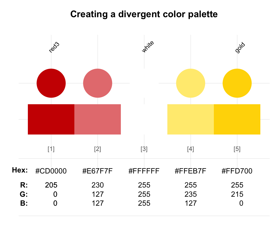

See the newpal() and usecol() functions of the unikn package for additional examples.

10.2.3 Working with colors in R

Here are some common color-related tasks for which we would like corresponding solutions (in the form of simple tools or recipes):

• See (or evaluate) a color or color palette

• Use a color or color palette (in a visualization)

• Change a color palette (number, order, transparency, vs. hue)

• Search for specific (parts of) color names

• Search for colors that are similar to a given color

Corresponding functions and instructions for solving these tasks can be found in the vignette on Color recipes of the unikn package.

10.3 Conclusion

When you really understand that each color is changed by a changed environment,
you eventually find that you have learned about life as well as about color.

Josef Albers

Colors can be arranged and classified, or systematically analyzed, defined and understood, but ultimately remain to be experienced. As their appearance changes based on their environment, even expert designers must first apply and view a concrete example to evaluate the effects of a color scheme for a particular task.

Artists and scientists have long been fascinated by the tension between the systematic study of colors and their chimeric flexibility. Explorations of their interactive and ephemeral nature have inspired many important works of art. In 1966, the German artist Gerhard Richter recognized the pictorial quality of industrial color sample cards and began using them as templates for ready-made works of art. His pioneering abstract work, 192 Farben (created in 1966), was recently sold for £18,287,800 (at Sotheby’s on 2022-10-14).

10.3.1 Summary

Colors are curious entities. Whereas most of us perceive and use them in an intuitive fashion, their representation can be both fascinating and confusing.

We distinguished between three basic ways of accessing colors in R:

1. The grDevices package defines and provides access to the 3 enumerated colors of palette() or the 657 named colors of colors(). These colors can easily be accessed by their name, but can be difficult to combine into pleasing color palettes.

2. Defining color objects by their RGB values (e.g., by using the rgb() function of the grDevices package).

3. Defining colors by their HEX values (as character objects with the prefix #), which are hexadecimal expressions of decimal RGB values (in the range from 0 to 255).

For a wider range of color palettes, we either use the palettes from dedicated color packages (like colorspace, RColorBrewer, unikn, scico or viridis) or construct our own color palettes (e.g., by using the usecol() and newpal() functions of unikn).

Some color packages (e.g., colorspace and unikn) contain additional functions for solving color-related tasks (like adjusting color transparency, creating color palettes, finding similar colors, or searching for color names).

10.3.2 Resources

See the following resources for a more solid introduction to color vision and color representation:

Books and articles

• The landmark publications by Jacques Bertin (e.g., Bertin, 2011) and some classic books by Edward Tufte (Tufte et al., 1990; Tufte, 2001, 2006) provide solid advice and many inspiring examples.

• More recent publications that are geared to the needs of aspiring data scientists include Healy (2018) and Wilke (2019).

• See Cleveland & McGill (1985) and Crameri et al. (2020) for the use and misuse of color in science communication.

• The following Wikipedia articles provide abundant background information:
  • Color model
  • Color vision
  • Color blindness
  • Color theory
  • Philosophy of color.

Online sites and tools

There is an abundance of online sites providing support for individual colors and color palettes. Examples include:

• HTML color picker provides HTML/HEX color codes.
• MyColor.space generates color palettes based on a single color.
• ColorBrewer 2.0 provides color support for cartography.
• MyColor.space generates nice color palettes from a base color
• Pantone color finder allows finding the color codes of many “official” colors.

Many sites collect color palettes and provide their definitions so that they can easily be implemented in various systems. Examples include:

• Color Lisa: Color palettes from art masterpieces (see the R package lisa)
• ColourLovers.com (see the R package colourlovers)
• ColorHunt.co
• Schemecolor.com (though many names seem dubious)
• Scientific colour maps

Color packages in R

We recommend and use the following R packages and resources:

• Popular and powerful color packages include: colorspace, RColorBrewer, and viridis/viridisLite.

• The ggsci and scico packages provide ordered and perceptually-uniform palettes for scientific visualizations.

• For more personal color choices, check out the colourlovers, rijkspalette, wesanderson, and yarrr packages.

• When dealing with maps and geographic data, consider using the color palettes from the RColorBrewer, viridis, or cartography packages.

• The unikn package provides the color palettes for the University of Konstanz, but also many useful functions for easily defining, modifying, and viewing color palettes, and for finding similar colors or color names.

• The paletteer package is a meta-color package that provides a uniform interface for palettes from many other packages.

Color-blind design

Just as architects must make public buildings accessible to all, new color desgins should be as inclusive and universal as possible. An important prerequisite for this is that visual designers know how different people perceive colors.

• See Okabe & Ito (2008) for an introduction to and recommendations for color universal design.

• The R packages colorspace, dichromat, viridis, and scico provide support for people with different color vision and allow simulating the effects of color-blindness.

• See the Wikipedia article on Color blindness for background information and links to additional resources.

Beware

As the wealth of color options are often overwhelming, please be aware of two final notes of caution:

• When defining or looking up colors, always double-check their specifications and names, and acknowledge your sources.

• While playing with colors can be fun, using color palettes designed by experts typically yields superior results over home-brew solutions.

10.3.3 Preview

These explorations of colors and color spaces conclude the part on visualizing data. As R plotting functions and packages that yield beautiful graphs typically assume that the data to be plotted is in a particular format, we often need to reshape our data before we can create beautiful and powerful visualizations. Thus, the next part and its chapters gravitate around different aspects of data transformation (i.e., getting, re-shaping, and reducing data).

10.4 Exercises

Here are some color-related exercises. Note that many of these exercises can be solved by using the corresponding unikn functions (or functions from other R color packages). However, using the colors(), col2rgb() and rgb() functions of the grDevices package provides a more basic understanding of the underlying representations.

10.4.1 Color representations

1. Starting from R colors: Skimming the range of named colors() of grDevices:
   • Draw 2 random colors (or choose 2 colors with particularly exotic names, e.g., "honeydew" and "peachpuff").
   • Find out their RGB and HEX values and re-define both colors (as R objects with new color names).
   • Create a visualization that uses both colors.

Hint: Most of the color-related tasks can be performed by using the seecol() and demopal() functions of the unikn package. For a more basic approach, consider using the col2rgb() and rgb() functions of the grDevices package.

2. Starting from RGB values:
   • Define 2 colors with the RGB values of 255/105/180 and 179/238/58, respectively.
   • What are their corresponding HEX values?
   • What are their corresponding R names?

Hint: Use the rgb() function of the grDevices package for defining colors from RGB values (and remember to adjust maxColorValue). The simcol() function of unikn allows finding similar colors (within a specific tolerance range tol).

3. Starting from HEX values:
   • Define 2 colors with the HEX codes of 123ABC and ABC123, respectively.
   • Before visualizing the colors: Compute their corresponding RGB values (by converting hexadecimal into decimal values) and predict their appearance.
   • Create a visualization that uses both colors and verify your prediction.

Hint: It is straightforward to define color objects from HEX values in R (as character objects with the prefix #). Visualizing such objects with seecol() provides their RGB values and names (if names exist). Alternatively, the base2dec() function of ds4psy allows converting non-decimal (e.g., base-16) numeric sequences into decimal notation.

10.4.2 Following color recipes

1. Finding color names: How many colors with the letter sequence “red”, “green”, or “blue” in their name exit in colors()?

Hint: The grepal() function of unikn allows searching for color names in colors().

2. Finding similar colors: Which other named R color denotes the same color as "peru"?

Hint: The simcol() function of unikn allows finding similar colors (within a specific tolerance range tol).

10.4.3 Defining color palettes

1. Study the current range of University color palettes provided by the unicol package (Neth et al., 2023) (e.g., by studying unicol_data or the vignette on Color palettes). Then conduct an online search to find the official color definitions of some university not yet contained in unicol and define its colors as (a) new named color palette(s). (Make sure to include a reference to your online source.)

Hint: The newpal() function of unikn allows defining new named color palettes.

2. Bonus: Find an image with a characteristic color scheme (e.g., a commercial ad, movie poster, subway map, university color scheme, etc.) and recreate its characteristic colors as a color palette with named colors. Illustrate the use of your palette in a series of images and discuss its potential for being used in scientific visualizations.

Hint: Use an online color picker tool to identify the colors of an image.

Bonus exercises

The following exercises (marked as Bonus) are optional (i.e., not required for passing this course).

10.4.4 Bonus: The RGB color cube

The RGB color system provides a 3D-space for color values. Use R to create visualizations of either

• 1. six 2D-images of the sides of the 3D-cube (where one dimension is set either to its minimum or to its maximum value); or
• 2. one 3D-image showing the color of random points within the cube.

Hint: Use colored tiles to visualize locations in the 2D- or 3D-space.

10.4.5 Bonus: Demonstrating color palettes

Explore the color palettes and the demopal() function of the unikn package.

• Which types of color palettes are provided by the package?

• Which type of plot is suitable for illustrating which type of color palette? (Consider the number of colors, their relations to each other, and the opacity/transparency level.)

• Create an alternative R plot for illustrating a categorical color palette.

• Create an alternative R plot for illustrating a continuous color palette.

10.4.6 Bonus: Homage to Josef Albers

Study the Wikipedia entry on Josef Albers and the website of The Josef and Anni Albers Foundation, especially the parts on the series Homage to the Square (begun in 1949) and the Interaction of color (1963).

• Create an R plot of colored squares or the triangular color model of Albers’ color theory.

---

23. Josef Albers published a book Interaction of Color in 1963, but John Dewey’s Art as Experience dates back to 1934.↩︎

24. Strictly speaking, different shades of a given color can be further distinguished by different opacity or transparency levels (typically denoted by an alpha value). However, the visual appearance of a transparent color can be mimicked by mixing the color with the background color (usually “white”). Hence, transparent shades of a color are usually not counted as different colors.↩︎

25. Assuming no ideological reasons for using or avoiding particular names, such examples illustrate that the perception of color is constructed in the eyes and mind of the beholder.↩︎