D.4 Using color packages
Most packages that primarily deal with visualizations — like ggplot2, lattice, or plotly — provide their own color palettes. To reach beyond the 657 predefined colors of R and the color palettes included in grDevices, the primary resource are packages that provide additional — and typically more specialized — color support.
There is a large number of R packages that provide dedicated color support (i.e., define colors and color scales, and corresponding functions) for all means and purposes. As a consequence, many users of R never define a new color palette, but use the color palettes provided by others. However, to choose nice colors, we have to know which options exist and how they can be chosen and compared. As choosing colors is not just an art, but also a matter of taste, we merely mention some personal preferences in this section.
D.4.1 RColorBrewer
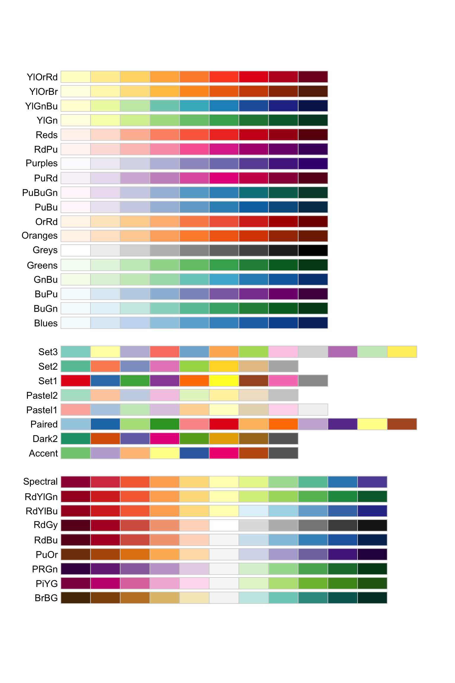
The colors at http://colorbrewer2.org (Brewer, 2019) were primarily designed to color maps. Beyond cartography, the vibrant color palettes are widely used in the R community, thanks to the popular RColorBrewer package (Neuwirth, 2022) and their integration into the ggplot2 package (Wickham, Chang, et al., 2025).
Actually, unless you happen to need very special colors, RColorBrewer provides nice and useful color palettes that are sufficient for most purposes.
The following command prints all color palettes included in RColorBrewer:
D.4.2 viridis/viridisLite
The color scales of the viridis package (Garnier, 2024) were specifically designed to be perceptually-uniform, both in regular form and when converted to black-and-white.
Its color palettes viridis, magma, plasma, and inferno can also be perceived by readers with the most common form of color blindness, and the cividis scale is even suited for people with color vision deficiency.
library(viridis)  # load package

x <- y <- seq(-8*pi, 8*pi, len = 40)
r <- sqrt(outer(x^2, y^2, "+"))
filled.contour(cos(r^2) * exp(-r/(2*pi)),
               axes = FALSE,
               color.palette = viridis,
               asp = 1)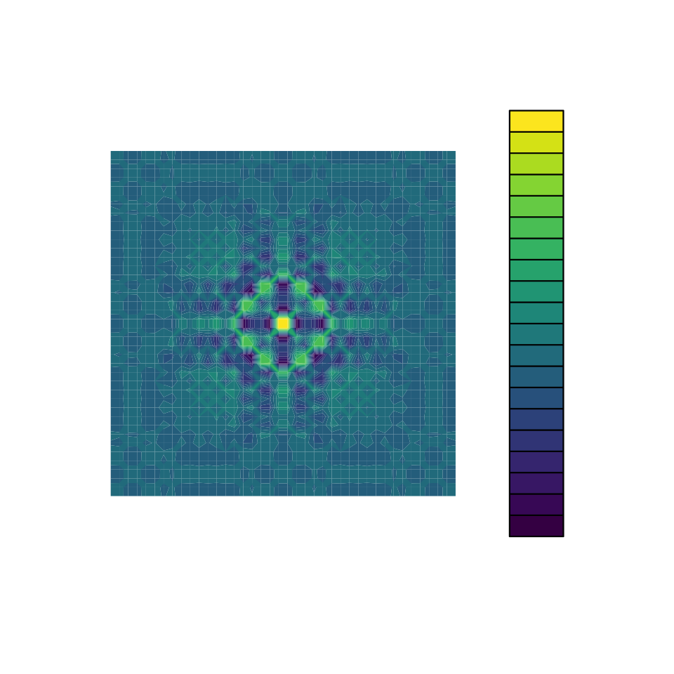
x <- y <- seq(-6*pi, 6*pi, len = 36)
r <- sqrt(outer(x^2, y^2, "+"))
filled.contour(cos(r^2) * exp(-r/(2*pi)),
               axes = FALSE,
               color.palette = inferno,
               asp = 1)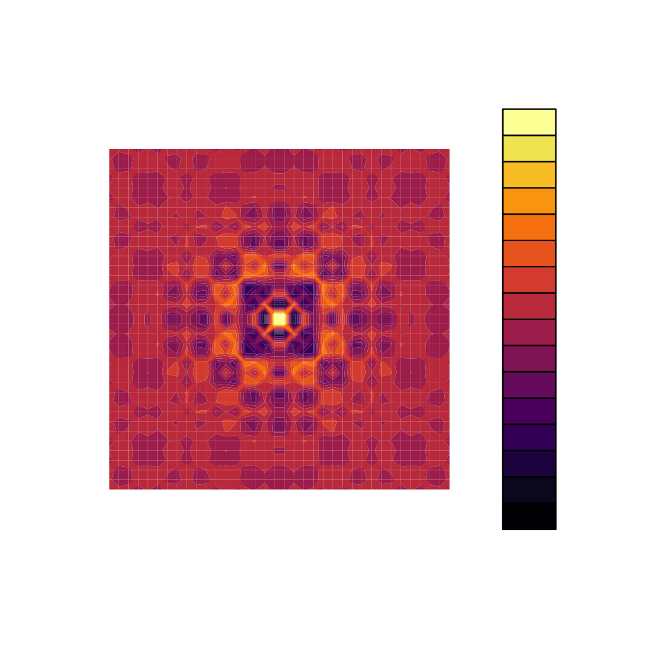
In recent versions of ggplot2, the viridis scales are integrated and can be used by specifying scale_color_viridis_c() and scale_color_viridis_c() (for continuous color scales) and scale_fill_viridis_d() and scale_fill_viridis_d() (for discrete color scales).
(See also Chapter 12.3 Using a Colorblind-Friendly Palette in the R Graphics Cookbook.)
The viridisLite package (Garnier, 2023) is a simpler version of the viridis package and sufficient for most purposes:
library(viridisLite)  # load package

vir_10 <- viridis(n = 10)
seecol(vir_10, col_brd = "white", lwd_brd = 4,
       main = "Example of a viridis color palette (n = 10)",
       pal_names = paste0("viridis_", 1:10))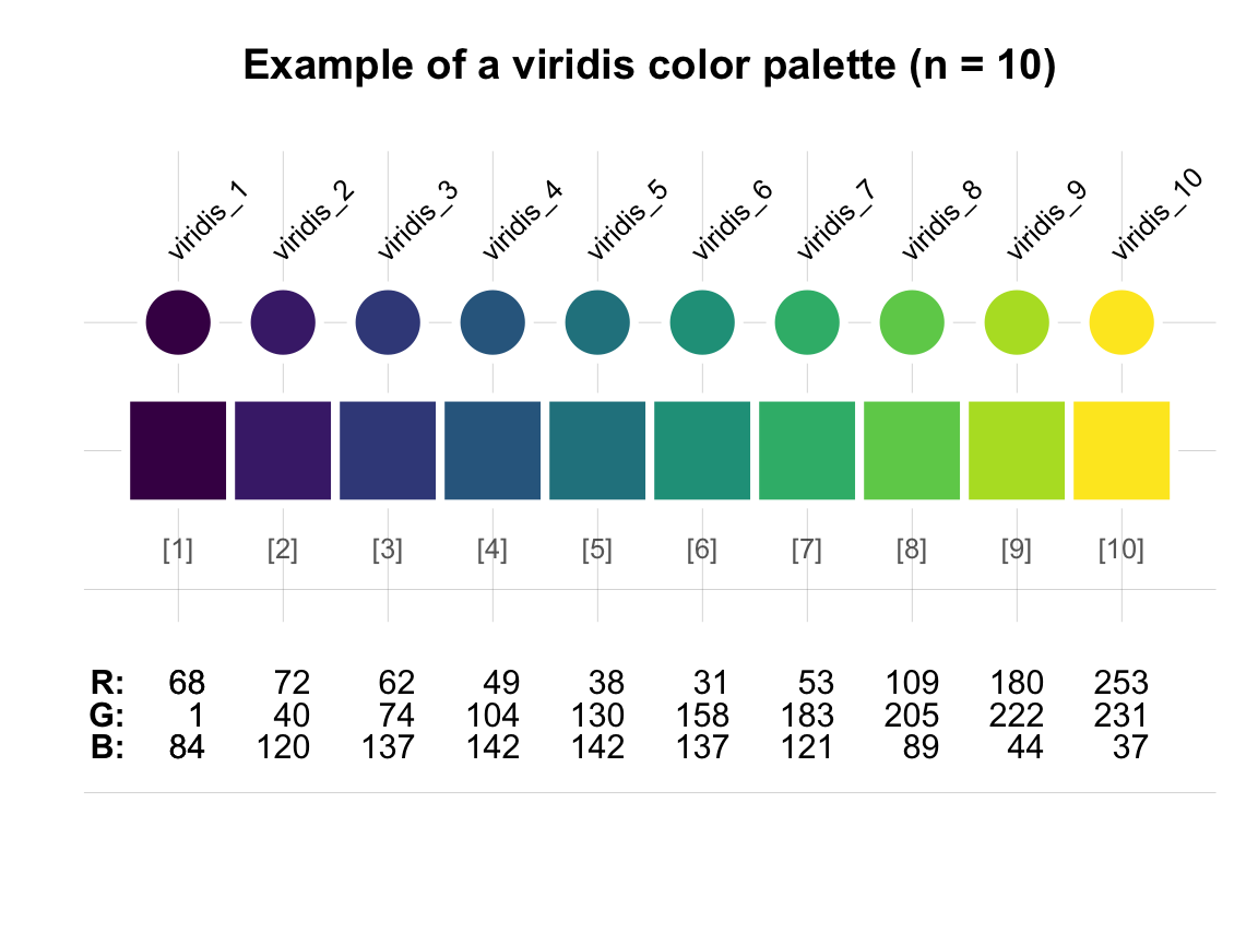
The following functions each define a color scale of n colors:
n <- 20  # number of colors

# define 5 different color scales (n colors each):
v1 <- viridis(n)
v2 <- magma(n)
v3 <- inferno(n)
v4 <- plasma(n)
v5 <- cividis(n)

# See and compare color scales:
seecol(list(v1, v2, v3, v4, v5),
       col_brd = "white", lwd_brd = 4,
       main = "Various viridis color palettes (n = 20)",
       pal_names = c("v1: viridis", "v2: magma", "v3: inferno", "v4: plasma",  "v5: cividis"))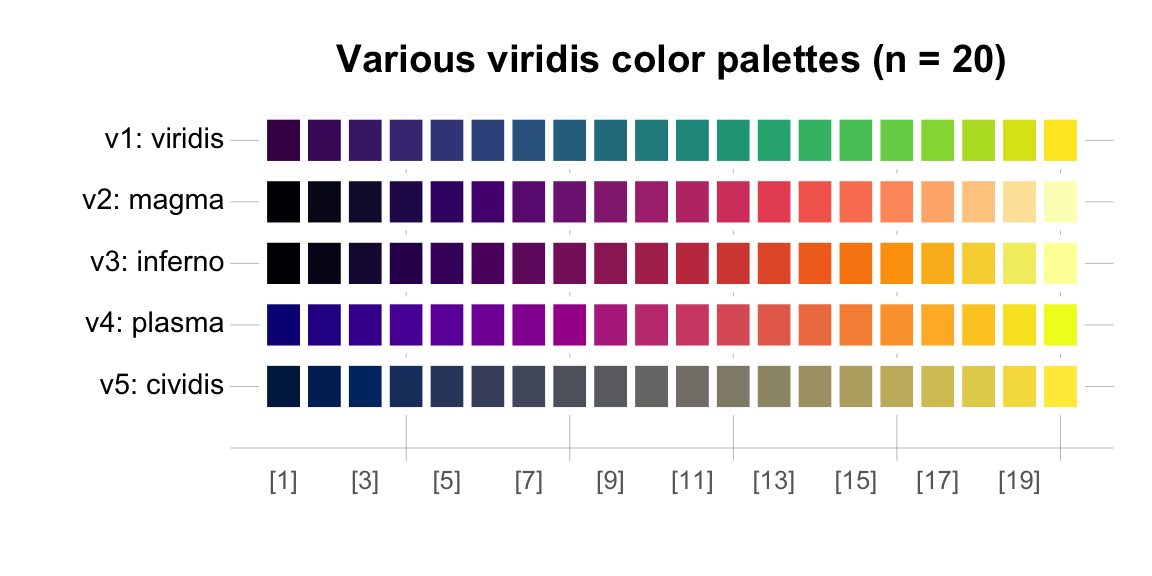
Check out ?viridisLite::viridis for additional information.
Another option for obtaining perceptually ordered and uniform color palettes are the Scientific colour maps by Fabio Crameri (F. Crameri, 2018). They are provided in many different formats — implemented by the scico package in R — friendly to people with color vision deficiency, and still readable in black-and-white print.
Finally, the dichromat package focuses on palettes for color-impaired viewers and allows simulating the effects of different types of color-blindness.
D.4.3 unikn
The unikn package (Neth & Gradwohl, 2024) implements the color palettes of the University of Konstanz and is used throughout this book. Additionally, the unicol package (Neth et al., 2025) provides the color palettes of many other universities and educational or research institutions.
Please note: As one of the authors of the unicol and unikn packages, I cannot help thinking that they are indispensable for working with colors. However, many people appear to live quite happy and colorful lives without ever needing these packages.
Besides providing some pre-defined color palettes, the unikn package provides color functions that are generally useful:
The
seecol()function allows a quick and easy inspections of color palettes. It has two distint modes, depending on the type of its first argumentpal:When called with a (single) color palette, it allows seeing (or printing the details of) a particular color palette;
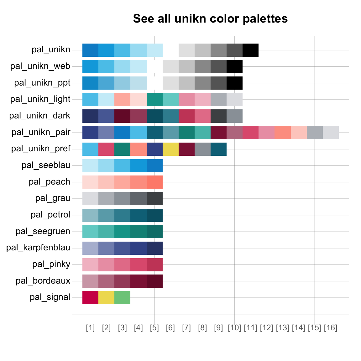
When called with a list of (several) color palettes or a recognized keyword, it allows comparing multiple color palettes.
Here are examples for seeing a single color palette:
library(unikn)  # load package
seecol(pal = pal_unikn)  # see/print details of a particular color palette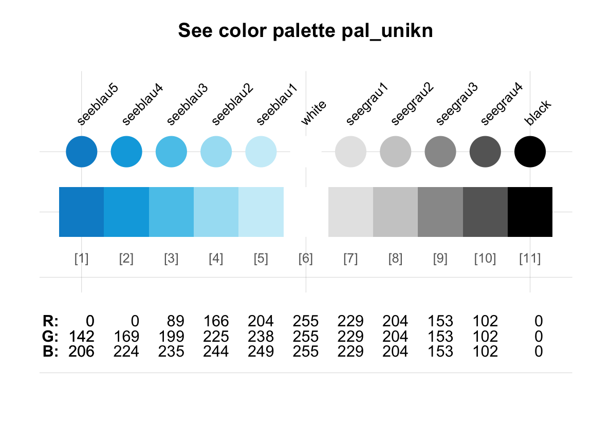
and for comparing several color palettes:
- The
usecol()function makes it easy to create new and modify existing color palettes. Its first argumentpalallows for vectors of colors or color palettes and its second argumentnallows to truncate or extend color palettes to a desired number of colors:
mix_1 <- usecol(pal = c(Karpfenblau, "white", Peach), n = 15)   # define color palette from 3 colors
mix_2 <- usecol(pal = c(rev(pal_seeblau), "white", pal_pinky))  # combining 2 color palettes
mix_3 <- usecol(pal = c(rev(pal_bordeaux), "white", pal_petrol), n = 15)  # mix and extend color palettes
To view and compare the three resulting color palettes, we can combine them in a list and visualize them with the seecol() function:
# Show and compare custom color palettes:
seecol(list(mix_1, mix_2, mix_3),
       col_brd = "white", lwd_brd = 4,
       main = "Comparing palettes mixed from unikn colors",
       pal_names = c("mix_1", "mix_2", "mix_3"))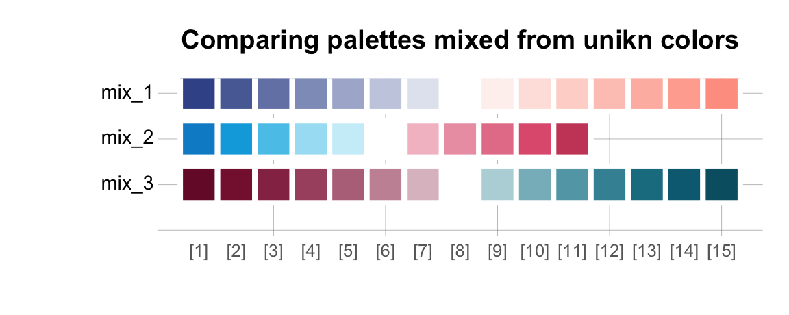
As colors in R can be represented in different data types and formats, the usecol() function also serves as a wrapper for using and modifying (pre-defined or newly created) color palettes in visualizations.
For instance, let’s use our gradient color palette mix_2 but stretch it to a range of n = 20 colors:
# Data:
x <- y <- seq(-8*pi, 8*pi, len = 40)
r <- sqrt(outer(x^2, y^2, "+"))

# Visualization:
filled.contour(cos(r^2) * exp(-r/(2*pi)),
               axes = FALSE,
               col = usecol(mix_2, n = 20),  # modify & use color palette
               asp = 1)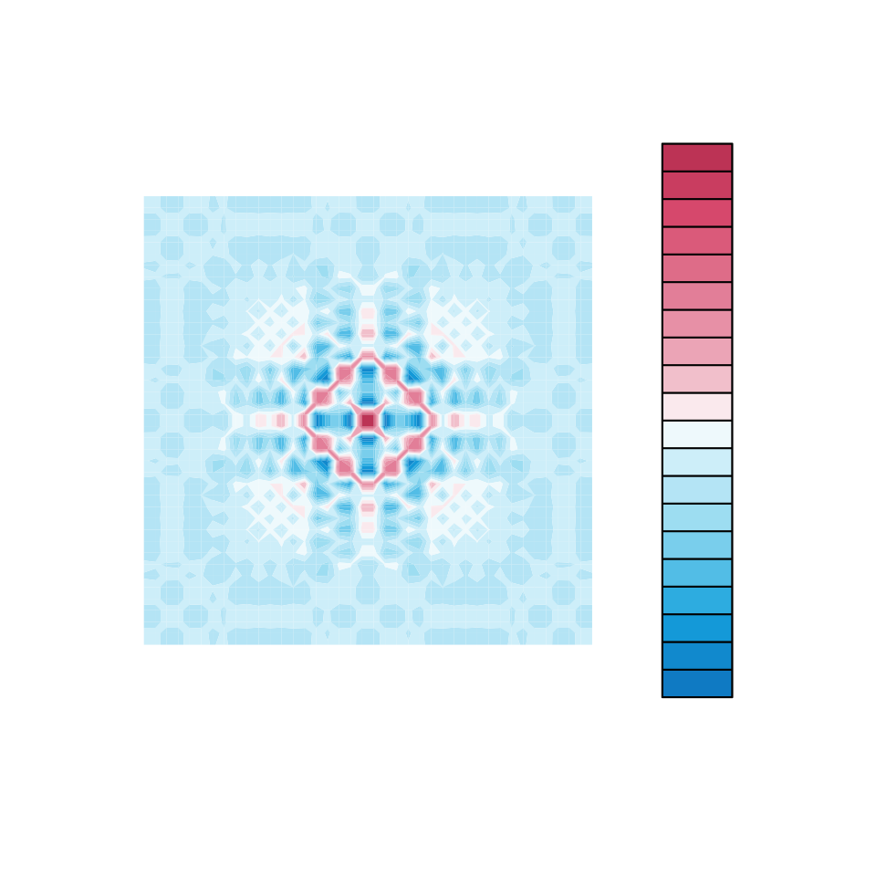
Even when not using the color palettes of the University of Konstanz, the usecol() and seecol() functions are often useful, as they also work with the color palettes provided by other packages.
For instance, we can use the seecol() function to compare (and modify) sets of color palettes from different packages.
In the following example, we first create 12 color palettes from three packages:
four color palettes from hcl.pals() of grDevices (R Core Team, 2025),
four color palettes from RColorBrewer (Neuwirth, 2022), and
four color palettes from yarrr (Phillips, 2025).
We then uses the seecol() function to view and compare all 12 color palettes:
# (a) get some HCL palettes (assuming R version 3.6.0+):
# hcl.pals() shows the names of all HCL palettes

hcl_1 <- hcl.colors(n = 10, palette = "Fall")
hcl_2 <- hcl.colors(n = 10, palette = "Geyser")
hcl_3 <- hcl.colors(n = 10, palette = "Berlin")
hcl_4 <- hcl.colors(n = 10, palette = "Zissou 1")


# (b) get some palettes from RColorBrewer:
library(RColorBrewer)
# display.brewer.all()  # shows all Brewer palettes

brew_1 <- brewer.pal(n = 11, name = "BrBG")
brew_2 <- brewer.pal(n = 11, name = "PRGn")
brew_3 <- brewer.pal(n = 11, name = "Spectral")
brew_4 <- brewer.pal(n = 8, name = "Pastel1")


# (c) get some palettes from yarrr:
library(yarrr)
# yarrr::piratepal()  # shows all pirate palettes

yarrr_1 <- yarrr::piratepal(palette = "basel")
yarrr_2 <- yarrr::piratepal(palette = "appletv")
yarrr_3 <- yarrr::piratepal(palette = "espresso")
yarrr_4 <- yarrr::piratepal(palette = "info")


my_pals <- list(hcl_1, hcl_2, hcl_3, hcl_4,
                brew_1, brew_2, brew_3, brew_4,
                yarrr_1, yarrr_2, yarrr_3, yarrr_4)
my_names <- c("hcl_1", "hcl_2", "hcl_3", "hcl_4",
              "brew_1", "brew_2", "brew_3", "brew_4",
              "yarrr_1", "yarrr_2", "yarrr_3", "yarrr_4")

# Show and compare color palettes:
library(unikn)
seecol(pal = my_pals,
       col_brd = "white", lwd_brd = 2,
       main = "Comparing HCL, RColorBrewer and yarrr color palettes",
       pal_names = my_names)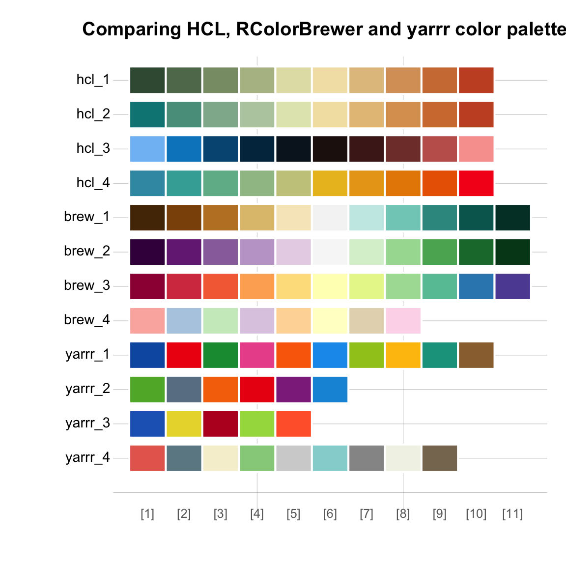
Similarly, we can use the usecol() function to mix and modify color palettes from various sources.
As before, it makes sense to inspect the results with seecol():
# Mix, extend and modify some palettes (from other packages):
brew_mix <- usecol(c(rev(  brewer.pal(n = 4, name = "Reds")),
                     "white", brewer.pal(n = 4, name = "Blues")), n = 13)
brew_ext <- usecol(brewer.pal(n = 11, name = "Spectral"), n = 12)

yarrr_mix <- usecol(c(piratepal("nemo"), piratepal("bugs")))
yarrr_mod <- usecol(c(piratepal("ipod")), n = 9)

my_pals <- list(brew_mix, brew_ext,
                yarrr_mix, yarrr_mod)
my_names <- c("brew_mix", "brew_ext",
              "yarrr_mix", "yarrr_mod")

# Show and compare new color palettes:
seecol(pal = my_pals,
       col_brd = "white", lwd_brd = 2,
       main = "Using usecol() and seecol() to mix and modify palettes",
       pal_names = my_names)
Additionally, the unikn package provides two functions that help with defining new named color palettes or finding colors with specific names:
- The
newpal()function makes it easy to define new named color palettes:
# (1) Source: <https://www.schemecolor.com/germany-flag-colors.php>
col_flag <- c("#000000", "#dd0000", "#ffce00")
names_de <- c("Black", "Electric red", "Tangerine yellow")

# (2) Source: <https://en.wikipedia.org/wiki/Flag_of_Germany#Design>
col_flag <- c("#000000", "#FF0000", "#FFCC00")
names_de <- c("Jet black", "Traffic red", "Rapeseed yellow")

# Decision: Simplify names:
simple_names <- c("de_black", "de_red", "de_gold")

# Define color palette:
flag_de  <- newpal(col = col_flag,
                   names = simple_names)

seecol(flag_de,
       main = "Defining a flag_de color palette",
       mar_note = "Colors based on <https://en.wikipedia.org/wiki/Flag_of_Germany>"  # credit source
       )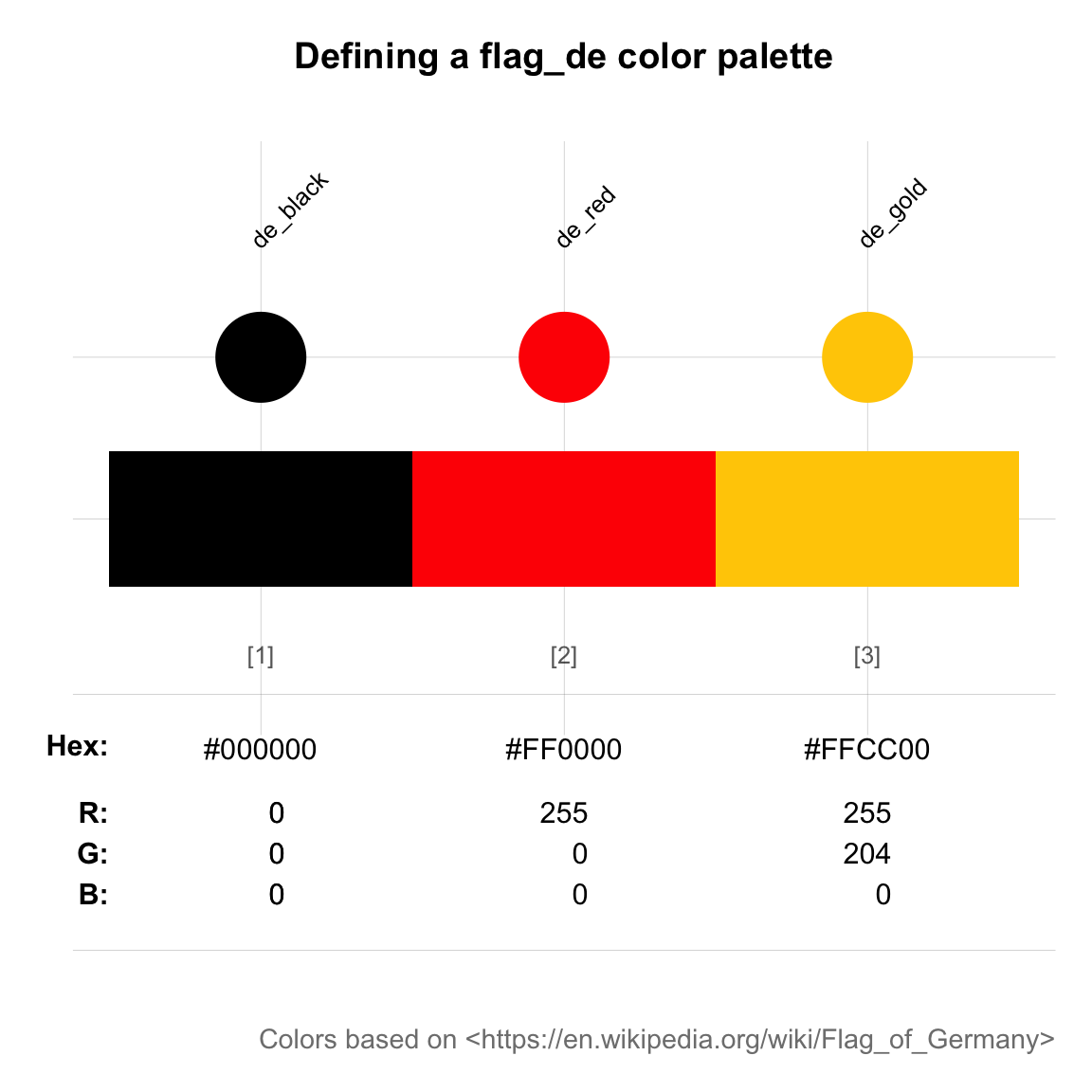
Note that different sources often provide different colors (and certainly different names) for the same color schemes. Thus, it always makes sense to double-check definitions and acknowledge one’s sources.
- The
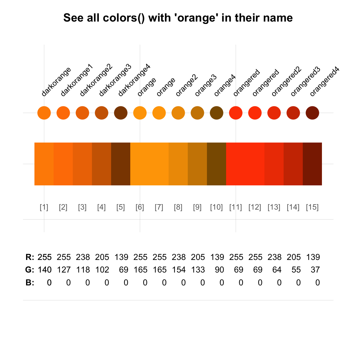
grepal()function of unikn addresses a common problem: We typically know that we want some shade of some color (e.g., orange), but do not know which corresponding color options exist in our environment. Thegrepal()function searches color names for a pattern:
grepal(pattern = "orange", plot = FALSE)  # returns colors() with "orange" in their name
#>  [1] "darkorange"  "darkorange1" "darkorange2" "darkorange3" "darkorange4"
#>  [6] "orange"      "orange1"     "orange2"     "orange3"     "orange4"
#> [11] "orangered"   "orangered1"  "orangered2"  "orangered3"  "orangered4"

seecol(pal = grepal("orange"),
       main = "See all colors() with 'orange' in their name")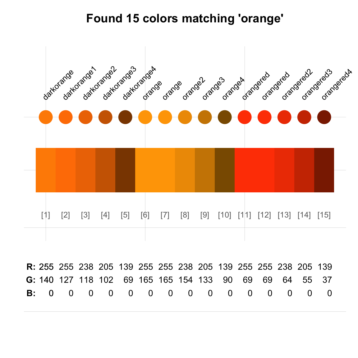
By default, grepal(pattern, x) searches x = colors() (i.e., the 657 named colors provided by the grDevices package), but x can be set to other named color palettes (including data frames). As pattern can be a regular expression (see Appendix E now provides a primer on using regular expressions), we can easily answer more complex questions:
Which color names end on pink, purple, or violet? How do these colors look?
How many shades of gray or grey are there (in R)?
Both these questions can easily be answered by combining two calls to the grepal() and the seecol() functions:
- Which color names end on pink, purple, or violet? How do these colors look?
cols_ppv <- grepal(pattern = "pink$|purple$|violet$", plot = FALSE)

seecol(pal = cols_ppv,
       main = "See all colors() with names ending on 'pink', 'purple' or 'violet'")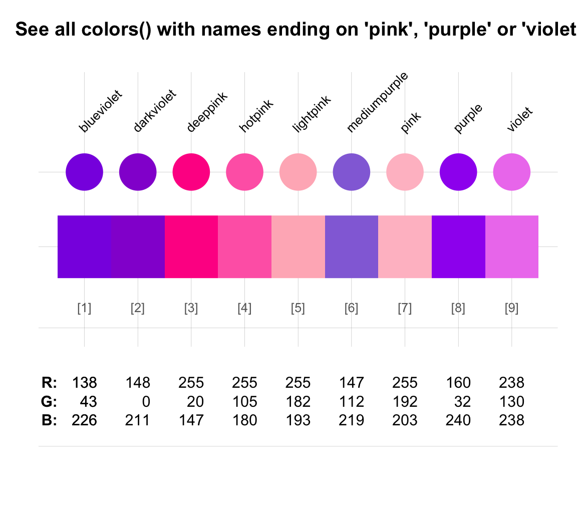
Actually, evaluating grepal(pattern = "pink$|purple$|violet$") would both return and show the corresponding colors.
- How many shades of gray or grey are there (in R)?
length(grepal("gr(a|e)y",   plot = FALSE))  # shades of "gray" or "grey"
#> [1] 224
length(grepal("^gr(a|e)y",  plot = FALSE))  # shades starting with "gray" or "grey"
#> [1] 204
length(grepal("^gr(a|e)y$", plot = FALSE))  # shades starting/ending with "gray" or "grey"
#> [1] 2
More generally, combining grepal() with seecol() allows creating and comparing color palettes containing certain keywords:
pal_r <- grepal("red",   plot = FALSE)
pal_g <- grepal("green", plot = FALSE)
pal_b <- grepal("blue",  plot = FALSE)

seecol(list(pal_r, pal_g, pal_b),
       main = "See all colors() with 'red', 'green', 'blue' in their name",
       pal_names = c('pal_r', 'pal_g', 'pal_b'))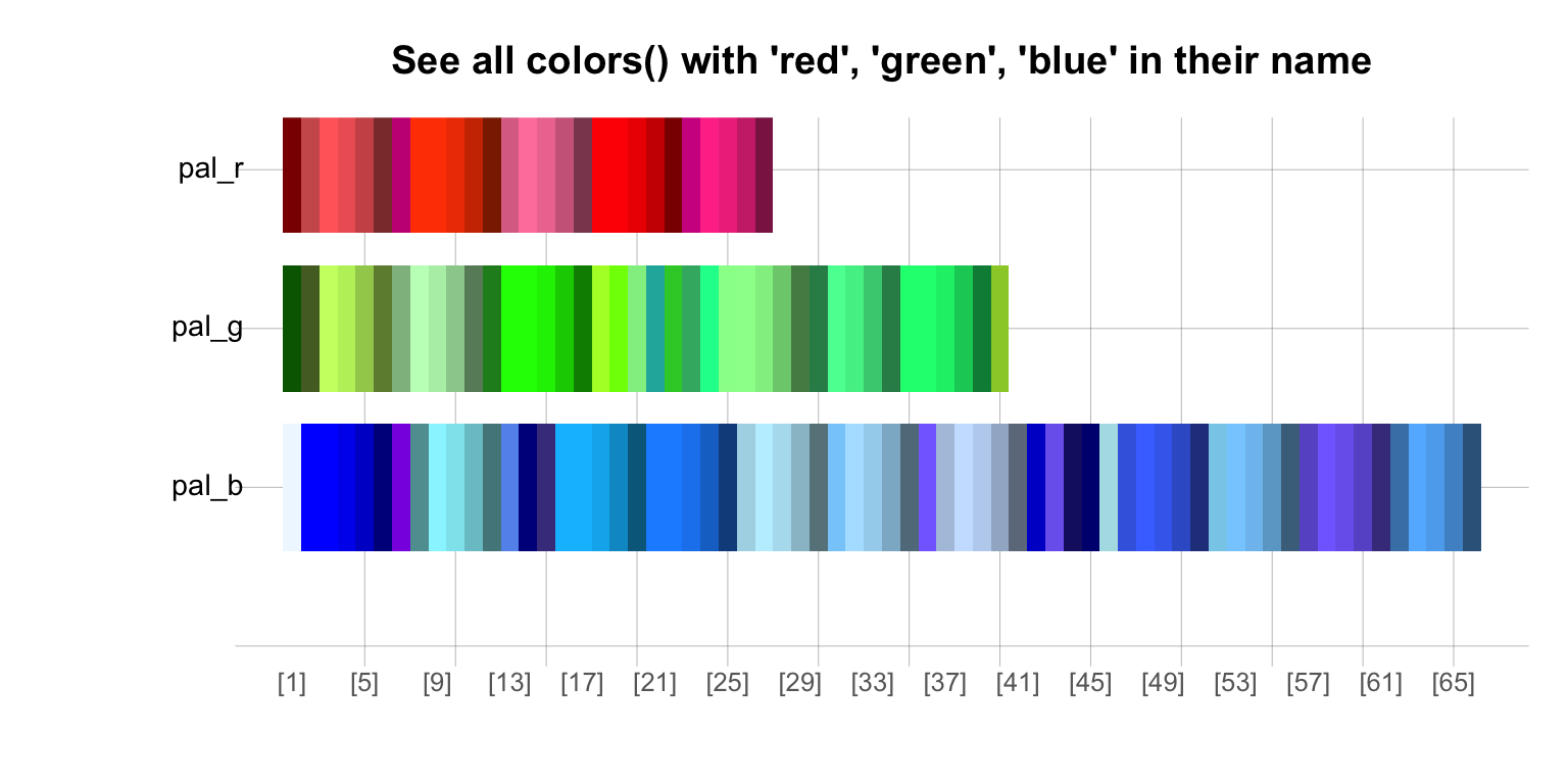
- The
simcol()function of unikn addresses a related and common problem: Given some color (e.g., “orange” or “#FFA500”), which similar colors exist in a set of candiate colors? Rather than searching for color names,simcol()searches for visually similar colors or existing colors with similar color values. By default, the set ofcol_candidatesis set to the 657colors()of grDevices:
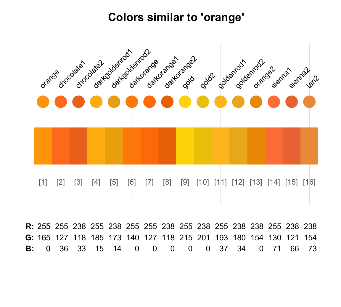
#>           orange       chocolate1       chocolate2   darkgoldenrod1
#>         "orange"     "chocolate1"     "chocolate2" "darkgoldenrod1"
#>   darkgoldenrod2       darkorange      darkorange1      darkorange2
#> "darkgoldenrod2"     "darkorange"    "darkorange1"    "darkorange2"
#>             gold            gold2       goldenrod1       goldenrod2
#>           "gold"          "gold2"     "goldenrod1"     "goldenrod2"
#>          orange2          sienna1          sienna2             tan2
#>        "orange2"        "sienna1"        "sienna2"           "tan2"
Setting the tol argument allows limiting and fine-tuning the range of color values (in RGB color space) that are considered to be similar:
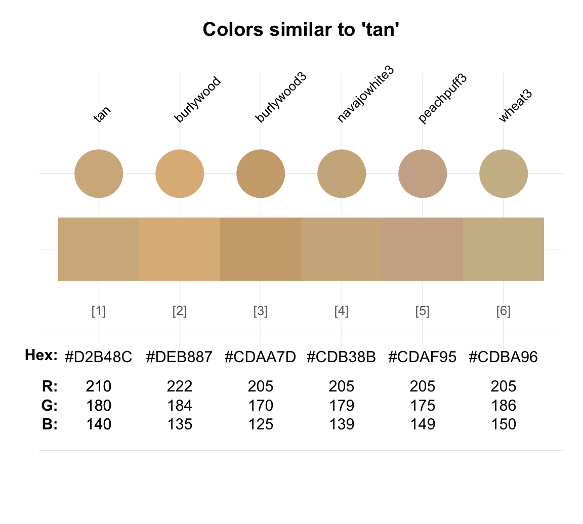
#>            tan      burlywood     burlywood3   navajowhite3     peachpuff3
#>          "tan"    "burlywood"   "burlywood3" "navajowhite3"   "peachpuff3"
#>         wheat3
#>       "wheat3"
simcol(Seeblau, tol = c(20, 20, 80))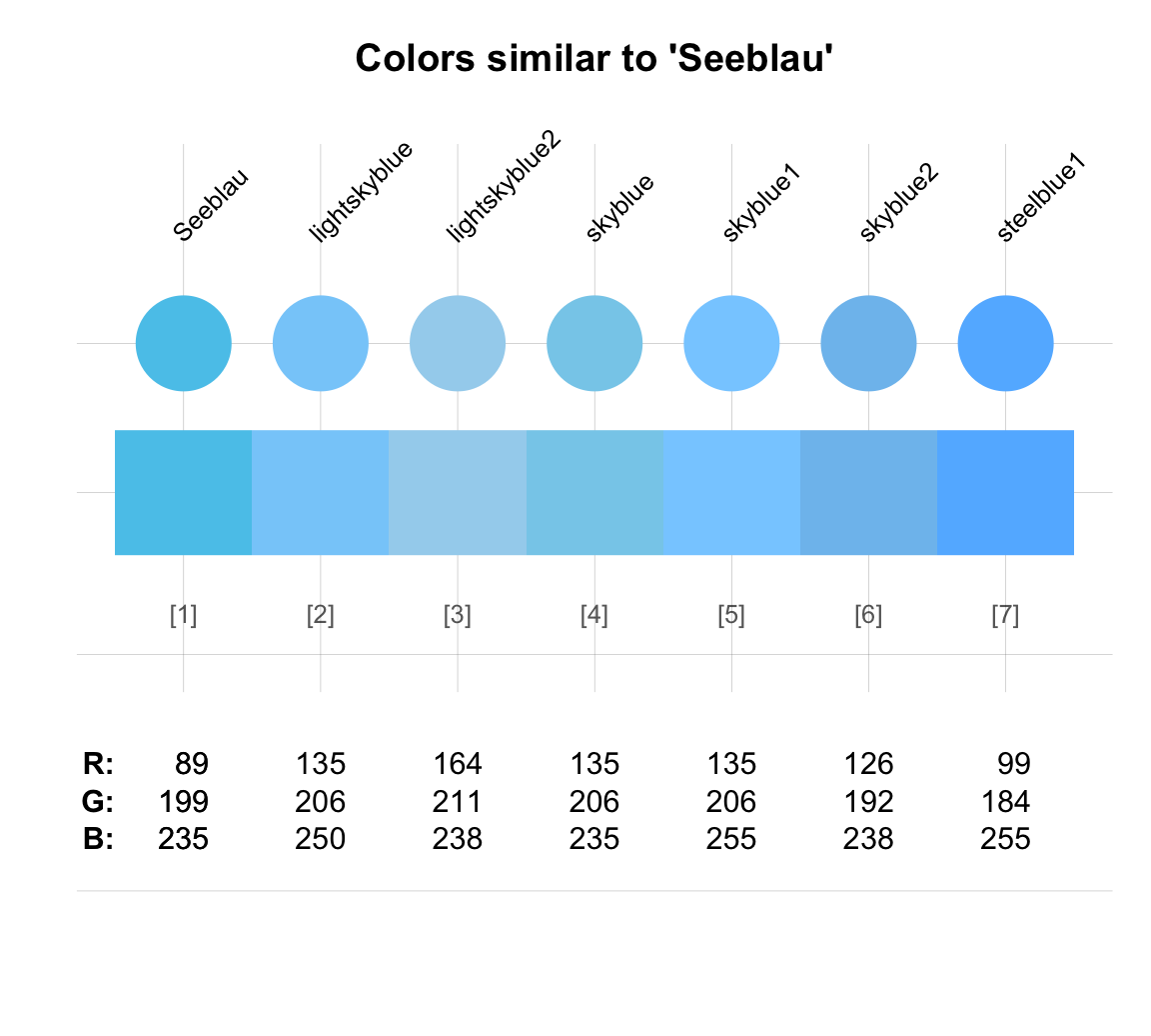
#>         Seeblau    lightskyblue   lightskyblue2         skyblue        skyblue1
#>       "#59C7EB"  "lightskyblue" "lightskyblue2"       "skyblue"      "skyblue1"
#>        skyblue2      steelblue1
#>      "skyblue2"    "steelblue1"
Finally, the color-related functions of the unikn package can be assembled into useful pipes by using the pipe operator %>% from the magrittr package (Bache & Wickham, 2025).
For instance, we can use multiple unikn functions to create and evaluate colorful chains of commands:
library(magrittr)

# Define and show a custom color palette:
cols <- c("#FAAB18", "#1380A1","#990000", "#588300")

cols %>%
  newpal(names = c("orangy", "bluish", "redish", "greeny")) %>%
  # usecol(n = 10) %>%
  seecol(main = "My new custom color palette")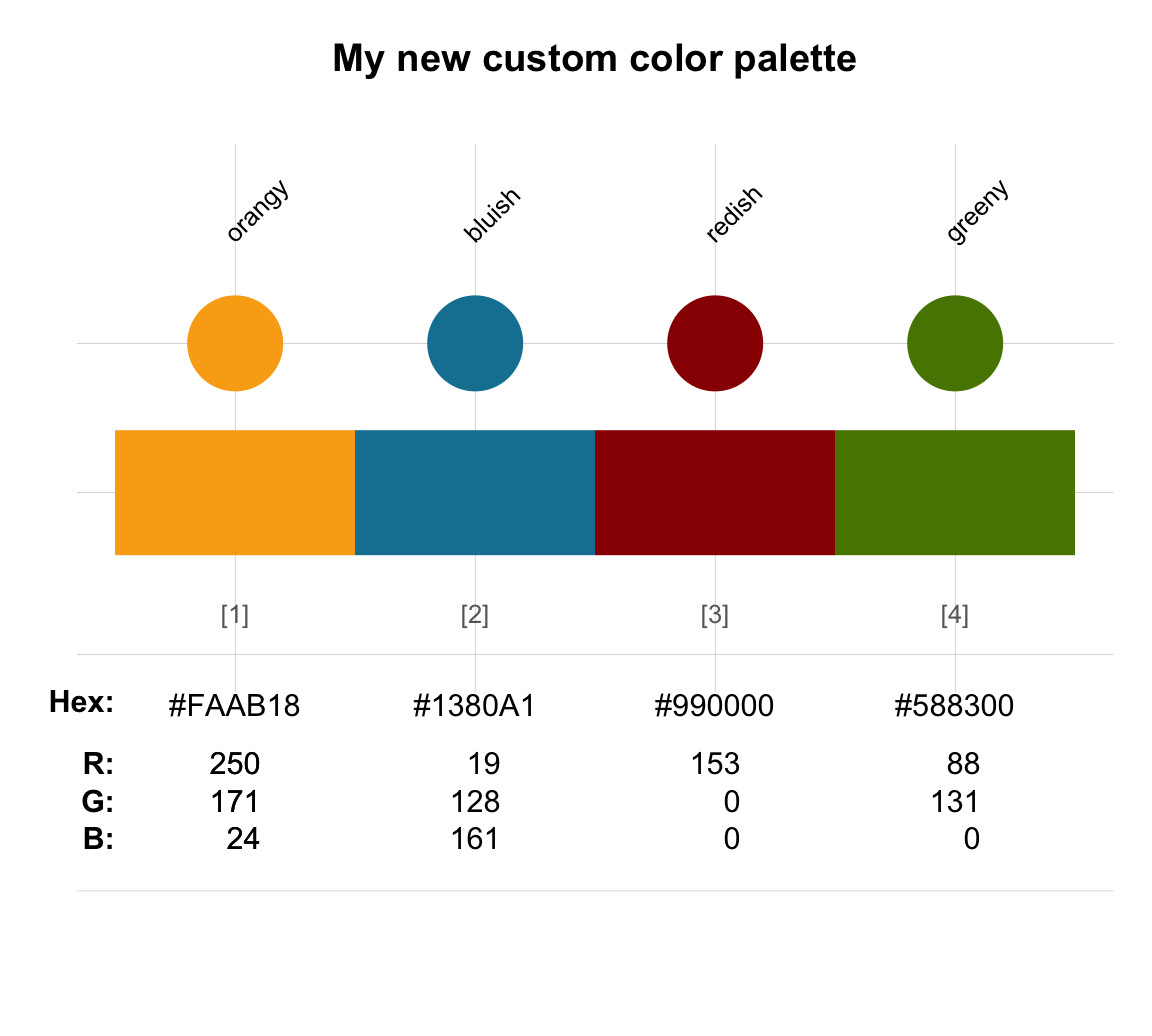
This concludes our overview of selected color packages in R. See Resources on color packages (in Section D.7.3) for links to many additional color packages.