3.2 Essential dplyr commands

Assuming that the dplyr package (Wickham, François, et al., 2023) is a toolbox for tackling various Rwars challenges, we can ask: Which specific tools does it provide and which tasks are addressed by them? In the context of this chapter, the following dplyr functions are essential for reshaping and reducing data:

arrange() sorts cases (rows);
filter() and slice() select cases (rows) by logical conditions or number;
select() selects and reorders variables (columns);
mutate() computes new variables (columns) and adds them to the existing ones;
summarise() collapses multiple values of a variable (rows of a column) to a single one;
group_by() and ungroup() change the unit of aggregation (in combination with mutate() and summarise()).

The following sections illustrate each of these commands in the context of examples. To keep things simple and entertaining, we use the toy dataset of sw <- dplyr::starwars to introduce the commands, but will use additional datasets in the exercises (in Section 3.5):

library(dplyr)  # load package
sw <- dplyr::starwars  # data

3.2.1 `arrange()` sorts rows

Using arrange() sorts cases (rows) by putting specific variables (columns) in specific orders (e.g., ascending or descending). For instance, we could want to arrange cases (rows) by the name of individuals (in alphabetical order). The dplyr function arrange() let’s us do this by calling:

# (a) Sort rows alphabetically (by name):
arrange(.data = sw, ... = name)

Before we proceed, two simple observations will facilitate our future life a lot:

In R, we can generally omit argument names (as long as the order of arguments makes it clear what is meant). Thus, we can write the same command more easily as:

# (b) Sort rows alphabetically (by name):
arrange(sw, name)

In dplyr and other tidyverse packages, we can rewrite commands by using the so-called pipe (written by the symbols %>%) of the magrittr package (Bache & Wickham, 2022):

# (c) Sort rows alphabetically (by name):
sw %>% arrange(name)

Think of the pipe as passing whatever is on its left (here: sw) to the first argument of the function on its right (here: .data). (More details about using the pipe operator are provided below in Section 3.3.)

In other words, the last three commands (a), (b), and (c) are identical and yield the same output:

#> # A tibble: 87 × 14
#>    name        height  mass hair_…¹ skin_…² eye_c…³ birth…⁴ sex   gender homew…⁵
#>    <chr>        <int> <dbl> <chr>   <chr>   <chr>     <dbl> <chr> <chr>  <chr>  
#>  1 Ackbar         180    83 none    brown … orange     41   male  mascu… Mon Ca…
#>  2 Adi Gallia     184    50 none    dark    blue       NA   fema… femin… Corusc…
#>  3 Anakin Sky…    188    84 blond   fair    blue       41.9 male  mascu… Tatooi…
#>  4 Arvel Cryn…     NA    NA brown   fair    brown      NA   male  mascu… <NA>   
#>  5 Ayla Secura    178    55 none    blue    hazel      48   fema… femin… Ryloth 
#>  6 Bail Prest…    191    NA black   tan     brown      67   male  mascu… Aldera…
#>  7 Barriss Of…    166    50 black   yellow  blue       40   fema… femin… Mirial 
#>  8 BB8             NA    NA none    none    black      NA   none  mascu… <NA>   
#>  9 Ben Quadin…    163    65 none    grey, … orange     NA   male  mascu… Tund   
#> 10 Beru White…    165    75 brown   light   blue       47   fema… femin… Tatooi…
#> # … with 77 more rows, 4 more variables: species <chr>, films <list>,
#> #   vehicles <list>, starships <list>, and abbreviated variable names
#> #   ¹hair_color, ²skin_color, ³eye_color, ⁴birth_year, ⁵homeworld

This output contains the tibble sw, but arranged the rows alphabetically by the variable name, which is exactly what we wanted. Although this is neat, two immediate questions are:

How can we arrange rows in different (e.g., descending, rather than ascending) orders?
How can we arrange rows by more than one variable?

Both of these tasks are solved rather intuitively by adjusting our calls to arrange():

# Sort rows in descending order:
sw %>% 
  arrange(desc(name))

#> # A tibble: 87 × 14
#>    name        height  mass hair_…¹ skin_…² eye_c…³ birth…⁴ sex   gender homew…⁵
#>    <chr>        <int> <dbl> <chr>   <chr>   <chr>     <dbl> <chr> <chr>  <chr>  
#>  1 Zam Wesell     168    55 blonde  fair, … yellow       NA fema… femin… Zolan  
#>  2 Yoda            66    17 white   green   brown       896 male  mascu… <NA>   
#>  3 Yarael Poof    264    NA none    white   yellow       NA male  mascu… Quermia
#>  4 Wilhuff Ta…    180    NA auburn… fair    blue         64 male  mascu… Eriadu 
#>  5 Wicket Sys…     88    20 brown   brown   brown         8 male  mascu… Endor  
#>  6 Wedge Anti…    170    77 brown   fair    hazel        21 male  mascu… Corell…
#>  7 Watto          137    NA black   blue, … yellow       NA male  mascu… Toydar…
#>  8 Wat Tambor     193    48 none    green,… unknown      NA male  mascu… Skako  
#>  9 Tion Medon     206    80 none    grey    black        NA male  mascu… Utapau 
#> 10 Taun We        213    NA none    grey    black        NA fema… femin… Kamino 
#> # … with 77 more rows, 4 more variables: species <chr>, films <list>,
#> #   vehicles <list>, starships <list>, and abbreviated variable names
#> #   ¹hair_color, ²skin_color, ³eye_color, ⁴birth_year, ⁵homeworld

# Sort by multiple variables:
sw %>% 
  arrange(eye_color, gender, desc(height))

#> # A tibble: 87 × 14
#>    name       height  mass hair_c…¹ skin_…² eye_c…³ birth…⁴ sex   gender homew…⁵
#>    <chr>       <int> <dbl> <chr>    <chr>   <chr>     <dbl> <chr> <chr>  <chr>  
#>  1 Taun We       213    NA none     grey    black        NA fema… femin… Kamino 
#>  2 Shaak Ti      178    57 none     red, b… black        NA fema… femin… Shili  
#>  3 Lama Su       229    88 none     grey    black        NA male  mascu… Kamino 
#>  4 Tion Medon    206    80 none     grey    black        NA male  mascu… Utapau 
#>  5 Kit Fisto     196    87 none     green   black        NA male  mascu… Glee A…
#>  6 Plo Koon      188    80 none     orange  black        22 male  mascu… Dorin  
#>  7 Greedo        173    74 <NA>     green   black        44 male  mascu… Rodia  
#>  8 Nien Nunb     160    68 none     grey    black        NA male  mascu… Sullust
#>  9 Gasgano       122    NA none     white,… black        NA male  mascu… Troiken
#> 10 BB8            NA    NA none     none    black        NA none  mascu… <NA>   
#> # … with 77 more rows, 4 more variables: species <chr>, films <list>,
#> #   vehicles <list>, starships <list>, and abbreviated variable names
#> #   ¹hair_color, ²skin_color, ³eye_color, ⁴birth_year, ⁵homeworld

See ?dplyr::arrange for more help and additional examples.

Details

Note some details on using arrange() in the above examples:

All basic dplyr commands can be called as verb(.data, ...) or — by using the pipe operator from magrittr — as .data %>% verb(...) (see vignette("magrittr") for details). Importantly, the pipe operator %>% is different from the + operator used in ggplot calls.
In contrast to base R commands, sequences of multiple variables in tidyverse commands can be written as comma-separated variables, rather than as vectors of variable names (e.g., c("gender", "height")) and are unquoted.
When specifying multiple variables in arrange, their order (x, y, ...) specifies the order or priority of operations (first by x, then by y, etc.).

Practice

Here are some exercises to practice using the dplyr verb arrange():

Arrange the sw data in different ways, combining multiple variables and (ascending and descending) orders.
Where are the cases containing missing (NA) values in sorted variables placed?

3.2.2 `filter()` selects rows

Using filter() selects cases (rows) by logical conditions or a criterion. It keeps all rows for which the criterion is TRUE and drops all rows for which the criterion is FALSE or NA.

For instance, two identical ways to extract all humans from sw are:

# Filter to keep all humans:
filter(sw, species == "Human")

# The same command using the pipe:
sw %>%           # Note: %>% is NOT + (used in ggplot) 
  filter(species == "Human")

and result in:

#> # A tibble: 35 × 14
#>    name        height  mass hair_…¹ skin_…² eye_c…³ birth…⁴ sex   gender homew…⁵
#>    <chr>        <int> <dbl> <chr>   <chr>   <chr>     <dbl> <chr> <chr>  <chr>  
#>  1 Luke Skywa…    172    77 blond   fair    blue       19   male  mascu… Tatooi…
#>  2 Darth Vader    202   136 none    white   yellow     41.9 male  mascu… Tatooi…
#>  3 Leia Organa    150    49 brown   light   brown      19   fema… femin… Aldera…
#>  4 Owen Lars      178   120 brown,… light   blue       52   male  mascu… Tatooi…
#>  5 Beru White…    165    75 brown   light   blue       47   fema… femin… Tatooi…
#>  6 Biggs Dark…    183    84 black   light   brown      24   male  mascu… Tatooi…
#>  7 Obi-Wan Ke…    182    77 auburn… fair    blue-g…    57   male  mascu… Stewjon
#>  8 Anakin Sky…    188    84 blond   fair    blue       41.9 male  mascu… Tatooi…
#>  9 Wilhuff Ta…    180    NA auburn… fair    blue       64   male  mascu… Eriadu 
#> 10 Han Solo       180    80 brown   fair    brown      29   male  mascu… Corell…
#> # … with 25 more rows, 4 more variables: species <chr>, films <list>,
#> #   vehicles <list>, starships <list>, and abbreviated variable names
#> #   ¹hair_color, ²skin_color, ³eye_color, ⁴birth_year, ⁵homeworld

To filter by some criterion (here: a test that determines whether species == "Human" is TRUE or FALSE), we needed to know both the variable by which we wanted to filter (here: species) and its value of interest (here: "Human"). Note that the output of applying filter to sw is a new tibble, but this tibble only contains 35 cases (i.e., the humans from sw).

Filtering by more than one condition can be very effective, but requires some knowledge about logical operators:

# Filter by multiple (additive) conditions: 
sw %>%
  filter(height > 180, mass <= 75)  # tall and light individuals

#> # A tibble: 3 × 14
#>   name         height  mass hair_…¹ skin_…² eye_c…³ birth…⁴ sex   gender homew…⁵
#>   <chr>         <int> <dbl> <chr>   <chr>   <chr>     <dbl> <chr> <chr>  <chr>  
#> 1 Jar Jar Bin…    196    66 none    orange  orange       52 male  mascu… Naboo  
#> 2 Adi Gallia      184    50 none    dark    blue         NA fema… femin… Corusc…
#> 3 Wat Tambor      193    48 none    green,… unknown      NA male  mascu… Skako  
#> # … with 4 more variables: species <chr>, films <list>, vehicles <list>,
#> #   starships <list>, and abbreviated variable names ¹hair_color, ²skin_color,
#> #   ³eye_color, ⁴birth_year, ⁵homeworld

# The same command using the logical operator (&): 
sw %>%
  filter(height > 180 & mass <= 75)  # tall and light individuals

#> # A tibble: 3 × 14
#>   name         height  mass hair_…¹ skin_…² eye_c…³ birth…⁴ sex   gender homew…⁵
#>   <chr>         <int> <dbl> <chr>   <chr>   <chr>     <dbl> <chr> <chr>  <chr>  
#> 1 Jar Jar Bin…    196    66 none    orange  orange       52 male  mascu… Naboo  
#> 2 Adi Gallia      184    50 none    dark    blue         NA fema… femin… Corusc…
#> 3 Wat Tambor      193    48 none    green,… unknown      NA male  mascu… Skako  
#> # … with 4 more variables: species <chr>, films <list>, vehicles <list>,
#> #   starships <list>, and abbreviated variable names ¹hair_color, ²skin_color,
#> #   ³eye_color, ⁴birth_year, ⁵homeworld

# Filter for a range of a specific variable:
sw %>%
  filter(height >= 150, height <= 165)  # (a) using height twice

#> # A tibble: 9 × 14
#>   name         height  mass hair_…¹ skin_…² eye_c…³ birth…⁴ sex   gender homew…⁵
#>   <chr>         <int> <dbl> <chr>   <chr>   <chr>     <dbl> <chr> <chr>  <chr>  
#> 1 Leia Organa     150    49 brown   light   brown        19 fema… femin… Aldera…
#> 2 Beru Whites…    165    75 brown   light   blue         47 fema… femin… Tatooi…
#> 3 Mon Mothma      150    NA auburn  fair    blue         48 fema… femin… Chandr…
#> 4 Nien Nunb       160    68 none    grey    black        NA male  mascu… Sullust
#> 5 Shmi Skywal…    163    NA black   fair    brown        72 fema… femin… Tatooi…
#> 6 Ben Quadina…    163    65 none    grey, … orange       NA male  mascu… Tund   
#> 7 Cordé           157    NA brown   light   brown        NA fema… femin… Naboo  
#> 8 Dormé           165    NA brown   light   brown        NA fema… femin… Naboo  
#> 9 Padmé Amida…    165    45 brown   light   brown        46 fema… femin… Naboo  
#> # … with 4 more variables: species <chr>, films <list>, vehicles <list>,
#> #   starships <list>, and abbreviated variable names ¹hair_color, ²skin_color,
#> #   ³eye_color, ⁴birth_year, ⁵homeworld

sw %>%
  filter(between(height, 150, 165))     # (b) using between(...)

#> # A tibble: 9 × 14
#>   name         height  mass hair_…¹ skin_…² eye_c…³ birth…⁴ sex   gender homew…⁵
#>   <chr>         <int> <dbl> <chr>   <chr>   <chr>     <dbl> <chr> <chr>  <chr>  
#> 1 Leia Organa     150    49 brown   light   brown        19 fema… femin… Aldera…
#> 2 Beru Whites…    165    75 brown   light   blue         47 fema… femin… Tatooi…
#> 3 Mon Mothma      150    NA auburn  fair    blue         48 fema… femin… Chandr…
#> 4 Nien Nunb       160    68 none    grey    black        NA male  mascu… Sullust
#> 5 Shmi Skywal…    163    NA black   fair    brown        72 fema… femin… Tatooi…
#> 6 Ben Quadina…    163    65 none    grey, … orange       NA male  mascu… Tund   
#> 7 Cordé           157    NA brown   light   brown        NA fema… femin… Naboo  
#> 8 Dormé           165    NA brown   light   brown        NA fema… femin… Naboo  
#> 9 Padmé Amida…    165    45 brown   light   brown        46 fema… femin… Naboo  
#> # … with 4 more variables: species <chr>, films <list>, vehicles <list>,
#> #   starships <list>, and abbreviated variable names ¹hair_color, ²skin_color,
#> #   ³eye_color, ⁴birth_year, ⁵homeworld

# Filter by multiple (alternative) conditions: 
sw %>%
  filter(homeworld == "Kashyyyk" | skin_color == "green")

#> # A tibble: 8 × 14
#>   name         height  mass hair_…¹ skin_…² eye_c…³ birth…⁴ sex   gender homew…⁵
#>   <chr>         <int> <dbl> <chr>   <chr>   <chr>     <dbl> <chr> <chr>  <chr>  
#> 1 Chewbacca       228   112 brown   unknown blue        200 male  mascu… Kashyy…
#> 2 Greedo          173    74 <NA>    green   black        44 male  mascu… Rodia  
#> 3 Yoda             66    17 white   green   brown       896 male  mascu… <NA>   
#> 4 Bossk           190   113 none    green   red          53 male  mascu… Trando…
#> 5 Rugor Nass      206    NA none    green   orange       NA male  mascu… Naboo  
#> 6 Kit Fisto       196    87 none    green   black        NA male  mascu… Glee A…
#> 7 Poggle the …    183    80 none    green   yellow       NA male  mascu… Geonos…
#> 8 Tarfful         234   136 brown   brown   blue         NA male  mascu… Kashyy…
#> # … with 4 more variables: species <chr>, films <list>, vehicles <list>,
#> #   starships <list>, and abbreviated variable names ¹hair_color, ²skin_color,
#> #   ³eye_color, ⁴birth_year, ⁵homeworld

A common criterion for filtering is that we want to (a) only obtain cases with missing values on some variable(s), or (b) only keep cases without missing values on some variable(s):

# (a) Filter cases with missing (NA) values on specific variables:
sw %>%
  filter(is.na(gender))

#> # A tibble: 4 × 14
#>   name         height  mass hair_…¹ skin_…² eye_c…³ birth…⁴ sex   gender homew…⁵
#>   <chr>         <int> <dbl> <chr>   <chr>   <chr>     <dbl> <chr> <chr>  <chr>  
#> 1 Ric Olié        183    NA brown   fair    blue         NA <NA>  <NA>   Naboo  
#> 2 Quarsh Pana…    183    NA black   dark    brown        62 <NA>  <NA>   Naboo  
#> 3 Sly Moore       178    48 none    pale    white        NA <NA>  <NA>   Umbara 
#> 4 Captain Pha…     NA    NA unknown unknown unknown      NA <NA>  <NA>   <NA>   
#> # … with 4 more variables: species <chr>, films <list>, vehicles <list>,
#> #   starships <list>, and abbreviated variable names ¹hair_color, ²skin_color,
#> #   ³eye_color, ⁴birth_year, ⁵homeworld

# (b) Filter cases with existing (non-NA) values on specific variables:
sw %>%
  filter(!is.na(mass), !is.na(birth_year))

#> # A tibble: 36 × 14
#>    name        height  mass hair_…¹ skin_…² eye_c…³ birth…⁴ sex   gender homew…⁵
#>    <chr>        <int> <dbl> <chr>   <chr>   <chr>     <dbl> <chr> <chr>  <chr>  
#>  1 Luke Skywa…    172    77 blond   fair    blue       19   male  mascu… Tatooi…
#>  2 C-3PO          167    75 <NA>    gold    yellow    112   none  mascu… Tatooi…
#>  3 R2-D2           96    32 <NA>    white,… red        33   none  mascu… Naboo  
#>  4 Darth Vader    202   136 none    white   yellow     41.9 male  mascu… Tatooi…
#>  5 Leia Organa    150    49 brown   light   brown      19   fema… femin… Aldera…
#>  6 Owen Lars      178   120 brown,… light   blue       52   male  mascu… Tatooi…
#>  7 Beru White…    165    75 brown   light   blue       47   fema… femin… Tatooi…
#>  8 Biggs Dark…    183    84 black   light   brown      24   male  mascu… Tatooi…
#>  9 Obi-Wan Ke…    182    77 auburn… fair    blue-g…    57   male  mascu… Stewjon
#> 10 Anakin Sky…    188    84 blond   fair    blue       41.9 male  mascu… Tatooi…
#> # … with 26 more rows, 4 more variables: species <chr>, films <list>,
#> #   vehicles <list>, starships <list>, and abbreviated variable names
#> #   ¹hair_color, ²skin_color, ³eye_color, ⁴birth_year, ⁵homeworld

As filter() selects cases, its result should typically be a table with the same number of columns as the original one, but fewer rows. See ?dplyr::filter for more help and additional examples.

Details

Note some details on using filter:

Separating multiple conditions by commas is the same as using the logical AND (&).
As seen with arrange(), variable names are unquoted.
A comma between conditions or tests (x, y, ...) means the same as & (logical AND), as each test results in a vector of Boolean values.
Unlike in base R, rows for which the condition evaluates to NA are dropped.
Additional filter functions include near() for testing numerical (near-)identity.

Practice

Here are some exercises to practice the combination of filter() and arrange() in dplyr pipes:

Verify for an example that filtering by two criteria yields the same result as filtering twice (once for each criterion).

# (a) Filtering by 2 criteria: 
tb1 <- sw %>% 
  filter(height >= 150, height <= 165) %>%
  arrange(name)

# (b) Filtering first by criterion 1, then by criterion 2: 
tb2 <- sw %>%
  filter(height >= 150) %>% 
  filter(height <= 165) %>%
  arrange(name) 

# (c) Filtering first by criterion 2, then by criterion 1: 
tb3 <- sw %>%
  filter(height <= 165) %>%
  filter(height >= 150) %>%
  arrange(name)

# Verify equality (of name variable):
all.equal(tb1$name, tb2$name)

#> [1] TRUE

all.equal(tb1$name, tb3$name)

#> [1] TRUE

Can you explain why we added arrange(name) to the end of each filter pipe?

Use filter() on the sw data to select some either diverse or narrow subset of individuals. For instance,

which individual with blond hair and blue eyes has an unknown mass?
of which species are individuals that are over 2m tall and have brown hair?
which individuals from Tatooine are not male (according to sex) but of masculine gender?
which individuals do neither identify as masculine nor as feminine (according to gender) OR are heavier than 150kg?

sw %>%
  filter(hair_color == "blond", eye_color == "blue")

sw %>%
  filter(height > 200, hair_color == "brown")

sw %>%
  filter(homeworld == "Tatooine", sex != "male", gender == "masculine")

sw %>%
  filter((gender != "masculine" & gender != "feminine") | mass > 150)

Note that the sw data distinguishes between an individual’s sex and gender.

`slice()` selects rows by number or value

If we want to select specific rows of a data table and already know their row number, we can use the slice() command of dplyr:

sw %>% slice(n = 2)           # the 2nd row

#> # A tibble: 1 × 14
#>   name  height  mass hair_color skin_color eye_co…¹ birth…² sex   gender homew…³
#>   <chr>  <int> <dbl> <chr>      <chr>      <chr>      <dbl> <chr> <chr>  <chr>  
#> 1 C-3PO    167    75 <NA>       gold       yellow       112 none  mascu… Tatooi…
#> # … with 4 more variables: species <chr>, films <list>, vehicles <list>,
#> #   starships <list>, and abbreviated variable names ¹eye_color, ²birth_year,
#> #   ³homeworld

sw %>% slice(n = 1:3)         # the first 3 rows

#> # A tibble: 3 × 14
#>   name         height  mass hair_…¹ skin_…² eye_c…³ birth…⁴ sex   gender homew…⁵
#>   <chr>         <int> <dbl> <chr>   <chr>   <chr>     <dbl> <chr> <chr>  <chr>  
#> 1 Luke Skywal…    172    77 blond   fair    blue         19 male  mascu… Tatooi…
#> 2 C-3PO           167    75 <NA>    gold    yellow      112 none  mascu… Tatooi…
#> 3 R2-D2            96    32 <NA>    white,… red          33 none  mascu… Naboo  
#> # … with 4 more variables: species <chr>, films <list>, vehicles <list>,
#> #   starships <list>, and abbreviated variable names ¹hair_color, ²skin_color,
#> #   ³eye_color, ⁴birth_year, ⁵homeworld

sw %>% slice(c(1, nrow(sw)))  # the 1st and last rows

#> # A tibble: 2 × 14
#>   name         height  mass hair_…¹ skin_…² eye_c…³ birth…⁴ sex   gender homew…⁵
#>   <chr>         <int> <dbl> <chr>   <chr>   <chr>     <dbl> <chr> <chr>  <chr>  
#> 1 Luke Skywal…    172    77 blond   fair    blue         19 male  mascu… Tatooi…
#> 2 Padmé Amida…    165    45 brown   light   brown        46 fema… femin… Naboo  
#> # … with 4 more variables: species <chr>, films <list>, vehicles <list>,
#> #   starships <list>, and abbreviated variable names ¹hair_color, ²skin_color,
#> #   ³eye_color, ⁴birth_year, ⁵homeworld

Several variants of slice() allow selecting a number n or proportion prop of all cases from the head or tail of a table, draw random samples of rows, or select the case(s) with the highest or lowest values on some variable:

sw %>% slice_head(prop = .05)  # top 5% of rows

#> # A tibble: 4 × 14
#>   name         height  mass hair_…¹ skin_…² eye_c…³ birth…⁴ sex   gender homew…⁵
#>   <chr>         <int> <dbl> <chr>   <chr>   <chr>     <dbl> <chr> <chr>  <chr>  
#> 1 Luke Skywal…    172    77 blond   fair    blue       19   male  mascu… Tatooi…
#> 2 C-3PO           167    75 <NA>    gold    yellow    112   none  mascu… Tatooi…
#> 3 R2-D2            96    32 <NA>    white,… red        33   none  mascu… Naboo  
#> 4 Darth Vader     202   136 none    white   yellow     41.9 male  mascu… Tatooi…
#> # … with 4 more variables: species <chr>, films <list>, vehicles <list>,
#> #   starships <list>, and abbreviated variable names ¹hair_color, ²skin_color,
#> #   ³eye_color, ⁴birth_year, ⁵homeworld

sw %>% slice_tail(n = 3)       # final 3 rows

#> # A tibble: 3 × 14
#>   name         height  mass hair_…¹ skin_…² eye_c…³ birth…⁴ sex   gender homew…⁵
#>   <chr>         <int> <dbl> <chr>   <chr>   <chr>     <dbl> <chr> <chr>  <chr>  
#> 1 BB8              NA    NA none    none    black        NA none  mascu… <NA>   
#> 2 Captain Pha…     NA    NA unknown unknown unknown      NA <NA>  <NA>   <NA>   
#> 3 Padmé Amida…    165    45 brown   light   brown        46 fema… femin… Naboo  
#> # … with 4 more variables: species <chr>, films <list>, vehicles <list>,
#> #   starships <list>, and abbreviated variable names ¹hair_color, ²skin_color,
#> #   ³eye_color, ⁴birth_year, ⁵homeworld

sw %>% slice_sample(n = 3)     # 3 random rows

#> # A tibble: 3 × 14
#>   name         height  mass hair_…¹ skin_…² eye_c…³ birth…⁴ sex   gender homew…⁵
#>   <chr>         <int> <dbl> <chr>   <chr>   <chr>     <dbl> <chr> <chr>  <chr>  
#> 1 Saesee Tiin     188    NA none    pale    orange       NA male  mascu… Iktotch
#> 2 Cliegg Lars     183    NA brown   fair    blue         82 male  mascu… Tatooi…
#> 3 Ki-Adi-Mundi    198    82 white   pale    yellow       92 male  mascu… Cerea  
#> # … with 4 more variables: species <chr>, films <list>, vehicles <list>,
#> #   starships <list>, and abbreviated variable names ¹hair_color, ²skin_color,
#> #   ³eye_color, ⁴birth_year, ⁵homeworld

sw %>% slice_max(mass)         # row(s) with highest mass

#> # A tibble: 1 × 14
#>   name         height  mass hair_…¹ skin_…² eye_c…³ birth…⁴ sex   gender homew…⁵
#>   <chr>         <int> <dbl> <chr>   <chr>   <chr>     <dbl> <chr> <chr>  <chr>  
#> 1 Jabba Desil…    175  1358 <NA>    green-… orange      600 herm… mascu… Nal Hu…
#> # … with 4 more variables: species <chr>, films <list>, vehicles <list>,
#> #   starships <list>, and abbreviated variable names ¹hair_color, ²skin_color,
#> #   ³eye_color, ⁴birth_year, ⁵homeworld

sw %>% slice_min(height)       # row(s) with lowest height

#> # A tibble: 1 × 14
#>   name  height  mass hair_color skin_color eye_co…¹ birth…² sex   gender homew…³
#>   <chr>  <int> <dbl> <chr>      <chr>      <chr>      <dbl> <chr> <chr>  <chr>  
#> 1 Yoda      66    17 white      green      brown        896 male  mascu… <NA>   
#> # … with 4 more variables: species <chr>, films <list>, vehicles <list>,
#> #   starships <list>, and abbreviated variable names ¹eye_color, ²birth_year,
#> #   ³homeworld

An R purist could point out that all functions of slice() and its variants can be replaced by base R indexing (or subsetting) functions. For instance, the expression sw[(nrow(sw) - 2):nrow(sw), ] would also select the final three rows of sw (see Section 1.5.3). Alternatively, we can replace many slice() commands by corresponding filter() expressions. For instance, we can create a column that contains the number of the corresponding row and then filter() for the numeric values of this column:

tb <- sw # copy data (to keep sw)

# Add a column that contains the row number:
tb$row_nr <- 1:nrow(sw)

# Apply filters (to the new column):
filter(tb, row_nr == 2)    # the 2nd row
filter(tb, row_nr == 1:3)  # the first 3 rows
filter(tb, row_nr == 1 | row_nr == nrow(sw))  # the 1st and last rows
filter(tb, row_nr %in% sample(1:nrow(tb), size = 3))  # 3 random rows

However, replacing slice() commands by their alternatives shows that the corresponding expressions can often get cumbersome and cryptic. As we will see throughout this book, R often provides many alternative ways of getting things done — and there is nothing wrong with having dedicated tools for solving simple tasks. Hence, slice() and its variants are a welcome addition to our dplyr vocabulary.

Practice

Here are some exercises to practice slicing our sw table:

Predict the outcome of slice(sw, 1:nrow(sw)) and then evaluate the expression and your prediction.

slice(sw, 1:nrow(sw))

Replace all instances of slice() and its variants above by subsetting sw or using filter() commands.

3.2.3 `select()` selects columns

Using select() selects variables (columns) by their names or numbers. As it works exactly like filter() (but selects columns, rather than rows), we can immediately select not just one, but multiple variables. Actually, there are many ways of achieving the same result:

# Select 4 specific variables (columns) of sw:
select(sw, name, species, birth_year, gender)

#> # A tibble: 87 × 4
#>    name               species birth_year gender   
#>    <chr>              <chr>        <dbl> <chr>    
#>  1 Luke Skywalker     Human         19   masculine
#>  2 C-3PO              Droid        112   masculine
#>  3 R2-D2              Droid         33   masculine
#>  4 Darth Vader        Human         41.9 masculine
#>  5 Leia Organa        Human         19   feminine 
#>  6 Owen Lars          Human         52   masculine
#>  7 Beru Whitesun lars Human         47   feminine 
#>  8 R5-D4              Droid         NA   masculine
#>  9 Biggs Darklighter  Human         24   masculine
#> 10 Obi-Wan Kenobi     Human         57   masculine
#> # … with 77 more rows

# The same when using the pipe:
sw %>%           # Note: %>% is NOT + (used in ggplot) 
  select(name, species, birth_year, gender)

#> # A tibble: 87 × 4
#>    name               species birth_year gender   
#>    <chr>              <chr>        <dbl> <chr>    
#>  1 Luke Skywalker     Human         19   masculine
#>  2 C-3PO              Droid        112   masculine
#>  3 R2-D2              Droid         33   masculine
#>  4 Darth Vader        Human         41.9 masculine
#>  5 Leia Organa        Human         19   feminine 
#>  6 Owen Lars          Human         52   masculine
#>  7 Beru Whitesun lars Human         47   feminine 
#>  8 R5-D4              Droid         NA   masculine
#>  9 Biggs Darklighter  Human         24   masculine
#> 10 Obi-Wan Kenobi     Human         57   masculine
#> # … with 77 more rows

# The same when providing a vector of variable names: 
sw %>%
  select(c(name, species, birth_year, gender))

#> # A tibble: 87 × 4
#>    name               species birth_year gender   
#>    <chr>              <chr>        <dbl> <chr>    
#>  1 Luke Skywalker     Human         19   masculine
#>  2 C-3PO              Droid        112   masculine
#>  3 R2-D2              Droid         33   masculine
#>  4 Darth Vader        Human         41.9 masculine
#>  5 Leia Organa        Human         19   feminine 
#>  6 Owen Lars          Human         52   masculine
#>  7 Beru Whitesun lars Human         47   feminine 
#>  8 R5-D4              Droid         NA   masculine
#>  9 Biggs Darklighter  Human         24   masculine
#> 10 Obi-Wan Kenobi     Human         57   masculine
#> # … with 77 more rows

# The same when providing column numbers:
sw %>%
  select(1, 10, 7, 8)

#> # A tibble: 87 × 4
#>    name               homeworld birth_year sex   
#>    <chr>              <chr>          <dbl> <chr> 
#>  1 Luke Skywalker     Tatooine        19   male  
#>  2 C-3PO              Tatooine       112   none  
#>  3 R2-D2              Naboo           33   none  
#>  4 Darth Vader        Tatooine        41.9 male  
#>  5 Leia Organa        Alderaan        19   female
#>  6 Owen Lars          Tatooine        52   male  
#>  7 Beru Whitesun lars Tatooine        47   female
#>  8 R5-D4              Tatooine        NA   none  
#>  9 Biggs Darklighter  Tatooine        24   male  
#> 10 Obi-Wan Kenobi     Stewjon         57   male  
#> # … with 77 more rows

# The same when providing a vector of column numbers: 
sw %>%
  select(c(1, 10, 7, 8))

#> # A tibble: 87 × 4
#>    name               homeworld birth_year sex   
#>    <chr>              <chr>          <dbl> <chr> 
#>  1 Luke Skywalker     Tatooine        19   male  
#>  2 C-3PO              Tatooine       112   none  
#>  3 R2-D2              Naboo           33   none  
#>  4 Darth Vader        Tatooine        41.9 male  
#>  5 Leia Organa        Alderaan        19   female
#>  6 Owen Lars          Tatooine        52   male  
#>  7 Beru Whitesun lars Tatooine        47   female
#>  8 R5-D4              Tatooine        NA   none  
#>  9 Biggs Darklighter  Tatooine        24   male  
#> 10 Obi-Wan Kenobi     Stewjon         57   male  
#> # … with 77 more rows

When selecting ranges of variables, the : operator allows selecting ranges of variables:

# Select ranges of variables with ":":
sw %>%
  select(name:mass, gender:species)

#> # A tibble: 87 × 6
#>    name               height  mass gender    homeworld species
#>    <chr>               <int> <dbl> <chr>     <chr>     <chr>  
#>  1 Luke Skywalker        172    77 masculine Tatooine  Human  
#>  2 C-3PO                 167    75 masculine Tatooine  Droid  
#>  3 R2-D2                  96    32 masculine Naboo     Droid  
#>  4 Darth Vader           202   136 masculine Tatooine  Human  
#>  5 Leia Organa           150    49 feminine  Alderaan  Human  
#>  6 Owen Lars             178   120 masculine Tatooine  Human  
#>  7 Beru Whitesun lars    165    75 feminine  Tatooine  Human  
#>  8 R5-D4                  97    32 masculine Tatooine  Droid  
#>  9 Biggs Darklighter     183    84 masculine Tatooine  Human  
#> 10 Obi-Wan Kenobi        182    77 masculine Stewjon   Human  
#> # … with 77 more rows

Selecting can also be used to re-arrange variables. In this case, the function everything() is useful, and refers to every variable not already specified:

# Select to re-order variables (columns) with everything():
sw %>%
  select(species, name, gender, everything())

#> # A tibble: 87 × 14
#>    species name        gender height  mass hair_…¹ skin_…² eye_c…³ birth…⁴ sex  
#>    <chr>   <chr>       <chr>   <int> <dbl> <chr>   <chr>   <chr>     <dbl> <chr>
#>  1 Human   Luke Skywa… mascu…    172    77 blond   fair    blue       19   male 
#>  2 Droid   C-3PO       mascu…    167    75 <NA>    gold    yellow    112   none 
#>  3 Droid   R2-D2       mascu…     96    32 <NA>    white,… red        33   none 
#>  4 Human   Darth Vader mascu…    202   136 none    white   yellow     41.9 male 
#>  5 Human   Leia Organa femin…    150    49 brown   light   brown      19   fema…
#>  6 Human   Owen Lars   mascu…    178   120 brown,… light   blue       52   male 
#>  7 Human   Beru White… femin…    165    75 brown   light   blue       47   fema…
#>  8 Droid   R5-D4       mascu…     97    32 <NA>    white,… red        NA   none 
#>  9 Human   Biggs Dark… mascu…    183    84 black   light   brown      24   male 
#> 10 Human   Obi-Wan Ke… mascu…    182    77 auburn… fair    blue-g…    57   male 
#> # … with 77 more rows, 4 more variables: homeworld <chr>, films <list>,
#> #   vehicles <list>, starships <list>, and abbreviated variable names
#> #   ¹hair_color, ²skin_color, ³eye_color, ⁴birth_year

A number of additional helper functions allow more sophisticated selections by testing variable names:

# Select variables with helper functions:
sw %>%
  select(starts_with("s"))

#> # A tibble: 87 × 4
#>    skin_color  sex    species starships
#>    <chr>       <chr>  <chr>   <list>   
#>  1 fair        male   Human   <chr [2]>
#>  2 gold        none   Droid   <chr [0]>
#>  3 white, blue none   Droid   <chr [0]>
#>  4 white       male   Human   <chr [1]>
#>  5 light       female Human   <chr [0]>
#>  6 light       male   Human   <chr [0]>
#>  7 light       female Human   <chr [0]>
#>  8 white, red  none   Droid   <chr [0]>
#>  9 light       male   Human   <chr [1]>
#> 10 fair        male   Human   <chr [5]>
#> # … with 77 more rows

sw %>%
  select(ends_with("s"))

#> # A tibble: 87 × 5
#>     mass species films     vehicles  starships
#>    <dbl> <chr>   <list>    <list>    <list>   
#>  1    77 Human   <chr [5]> <chr [2]> <chr [2]>
#>  2    75 Droid   <chr [6]> <chr [0]> <chr [0]>
#>  3    32 Droid   <chr [7]> <chr [0]> <chr [0]>
#>  4   136 Human   <chr [4]> <chr [0]> <chr [1]>
#>  5    49 Human   <chr [5]> <chr [1]> <chr [0]>
#>  6   120 Human   <chr [3]> <chr [0]> <chr [0]>
#>  7    75 Human   <chr [3]> <chr [0]> <chr [0]>
#>  8    32 Droid   <chr [1]> <chr [0]> <chr [0]>
#>  9    84 Human   <chr [1]> <chr [0]> <chr [1]>
#> 10    77 Human   <chr [6]> <chr [1]> <chr [5]>
#> # … with 77 more rows

sw %>%
  select(contains("_"))

#> # A tibble: 87 × 4
#>    hair_color    skin_color  eye_color birth_year
#>    <chr>         <chr>       <chr>          <dbl>
#>  1 blond         fair        blue            19  
#>  2 <NA>          gold        yellow         112  
#>  3 <NA>          white, blue red             33  
#>  4 none          white       yellow          41.9
#>  5 brown         light       brown           19  
#>  6 brown, grey   light       blue            52  
#>  7 brown         light       blue            47  
#>  8 <NA>          white, red  red             NA  
#>  9 black         light       brown           24  
#> 10 auburn, white fair        blue-gray       57  
#> # … with 77 more rows

sw %>%
  select(matches("or"))

#> # A tibble: 87 × 4
#>    hair_color    skin_color  eye_color homeworld
#>    <chr>         <chr>       <chr>     <chr>    
#>  1 blond         fair        blue      Tatooine 
#>  2 <NA>          gold        yellow    Tatooine 
#>  3 <NA>          white, blue red       Naboo    
#>  4 none          white       yellow    Tatooine 
#>  5 brown         light       brown     Alderaan 
#>  6 brown, grey   light       blue      Tatooine 
#>  7 brown         light       blue      Tatooine 
#>  8 <NA>          white, red  red       Tatooine 
#>  9 black         light       brown     Tatooine 
#> 10 auburn, white fair        blue-gray Stewjon  
#> # … with 77 more rows

The helper function where() allows applying a function to all variables and returns only those for which the function returns TRUE. For instance, if we wanted to only select numeric columns of sw, we could use:

sw %>% 
  select(where(is.numeric))

#> # A tibble: 87 × 3
#>    height  mass birth_year
#>     <int> <dbl>      <dbl>
#>  1    172    77       19  
#>  2    167    75      112  
#>  3     96    32       33  
#>  4    202   136       41.9
#>  5    150    49       19  
#>  6    178   120       52  
#>  7    165    75       47  
#>  8     97    32       NA  
#>  9    183    84       24  
#> 10    182    77       57  
#> # … with 77 more rows

The same could be achieved by using the select_if() variant of select():

sw %>% 
  select_if(is.numeric)

#> # A tibble: 87 × 3
#>    height  mass birth_year
#>     <int> <dbl>      <dbl>
#>  1    172    77       19  
#>  2    167    75      112  
#>  3     96    32       33  
#>  4    202   136       41.9
#>  5    150    49       19  
#>  6    178   120       52  
#>  7    165    75       47  
#>  8     97    32       NA  
#>  9    183    84       24  
#> 10    182    77       57  
#> # … with 77 more rows

As select() selects variables, its result should typically be a table with the same number of cases as the original one, but fewer columns, unless the variables specified include everything(). (See ?dplyr::select for more help and additional examples, as well as ?dplyr::select_if for conditional variants.)

Another dplyr function closely related to select() is rename(), which does exactly what it says:

# Renaming variables:
sw %>%
  rename(creature = name, from_planet = homeworld)

#> # A tibble: 87 × 14
#>    creature    height  mass hair_…¹ skin_…² eye_c…³ birth…⁴ sex   gender from_…⁵
#>    <chr>        <int> <dbl> <chr>   <chr>   <chr>     <dbl> <chr> <chr>  <chr>  
#>  1 Luke Skywa…    172    77 blond   fair    blue       19   male  mascu… Tatooi…
#>  2 C-3PO          167    75 <NA>    gold    yellow    112   none  mascu… Tatooi…
#>  3 R2-D2           96    32 <NA>    white,… red        33   none  mascu… Naboo  
#>  4 Darth Vader    202   136 none    white   yellow     41.9 male  mascu… Tatooi…
#>  5 Leia Organa    150    49 brown   light   brown      19   fema… femin… Aldera…
#>  6 Owen Lars      178   120 brown,… light   blue       52   male  mascu… Tatooi…
#>  7 Beru White…    165    75 brown   light   blue       47   fema… femin… Tatooi…
#>  8 R5-D4           97    32 <NA>    white,… red        NA   none  mascu… Tatooi…
#>  9 Biggs Dark…    183    84 black   light   brown      24   male  mascu… Tatooi…
#> 10 Obi-Wan Ke…    182    77 auburn… fair    blue-g…    57   male  mascu… Stewjon
#> # … with 77 more rows, 4 more variables: species <chr>, films <list>,
#> #   vehicles <list>, starships <list>, and abbreviated variable names
#> #   ¹hair_color, ²skin_color, ³eye_color, ⁴birth_year, ⁵from_planet

Note that rename() also uses (both old and new) variable names without enclosing them in quotation marks.

Details

Note some details on using select():

select() works both by specifying variable (column) names and by specifying column numbers.
Again, variable names are unquoted.
The sequence of variable names (separated by commas) specifies the order of columns in the resulting tibble.
Selecting and adding everything() allows re-ordering variables.
Various helper functions (e.g., starts_with, ends_with, contains, matches, num_range) refer to (parts of) variable names or apply functions to variables (e.g., where).
rename() renames specified variables (without quotes) and keeps all other variables.

Practice

Here are some exercises to practice the dplyr verbs encountered so far:

What is the result of sw %>% select(height)? More specifically, how does it differ from the vector sw$height?

x <- sw %>% select(height)
y <- sw$height 

# difference: 
is.vector(x)
is.vector(y)

Use select() or select_if() on the dplyr::starwars data (sw) to select and re-order specific subsets of variables (e.g., all variables starting with “h”, all even columns, all character variables, etc.).

sw %>% select(starts_with("h"))

even_col <- ((1:ncol(sw) %% 2) == 0)
sw %>% select_if(even_col)

sw %>% select(where(is.character))

Advanced: The dplyr command select(sw, where(is.numeric)) selects all numeric columns of a tibble sw. How could the same be achieved by using subsetting in base R?

Hint: As this turns out to be quite difficult, we will only cover the commands used here much later (in Chapter 12 on Iteration). This illustrates that dplyr enables us to solve tasks that would otherwise be much harder.

# (a) Using dplyr:
select(sw, where(is.numeric)) 
select_if(sw, is.numeric)

# (b) Using base R:
numeric_cols <- unlist(lapply(sw, is.numeric))  
sw[ , numeric_cols]

# (c) Using purrr: 
number_cols <- purrr::map_lgl(sw, is.numeric)
sw[ , number_cols]

3.2.4 `mutate()` computes new variables

Using mutate() computes new variables (columns) from scratch or existing ones. For instance, the height variable is provided in centimeters (cm). To transform this measure into feet, we need to divide it by 100 (to obtain height in meters) and multiply the result by a factor of 3.28084:

# Preparation: Save only a subset variables of sw as sws:   
sws <- select(sw, name:mass, birth_year:species) 
sws    # => 87 cases (rows), but only 7 variables (columns)

#> # A tibble: 87 × 8
#>    name               height  mass birth_year sex    gender    homeworld species
#>    <chr>               <int> <dbl>      <dbl> <chr>  <chr>     <chr>     <chr>  
#>  1 Luke Skywalker        172    77       19   male   masculine Tatooine  Human  
#>  2 C-3PO                 167    75      112   none   masculine Tatooine  Droid  
#>  3 R2-D2                  96    32       33   none   masculine Naboo     Droid  
#>  4 Darth Vader           202   136       41.9 male   masculine Tatooine  Human  
#>  5 Leia Organa           150    49       19   female feminine  Alderaan  Human  
#>  6 Owen Lars             178   120       52   male   masculine Tatooine  Human  
#>  7 Beru Whitesun lars    165    75       47   female feminine  Tatooine  Human  
#>  8 R5-D4                  97    32       NA   none   masculine Tatooine  Droid  
#>  9 Biggs Darklighter     183    84       24   male   masculine Tatooine  Human  
#> 10 Obi-Wan Kenobi        182    77       57   male   masculine Stewjon   Human  
#> # … with 77 more rows

# Conversion factor (cm to feet):
factor_cm_2_feet <- 3.28084/100

# Compute 2 new variables and add them to existing ones:
mutate(sws, id = 1:nrow(sw), 
            height_feet = factor_cm_2_feet * height)

#> # A tibble: 87 × 10
#>    name          height  mass birth…¹ sex   gender homew…² species    id heigh…³
#>    <chr>          <int> <dbl>   <dbl> <chr> <chr>  <chr>   <chr>   <int>   <dbl>
#>  1 Luke Skywalk…    172    77    19   male  mascu… Tatooi… Human       1    5.64
#>  2 C-3PO            167    75   112   none  mascu… Tatooi… Droid       2    5.48
#>  3 R2-D2             96    32    33   none  mascu… Naboo   Droid       3    3.15
#>  4 Darth Vader      202   136    41.9 male  mascu… Tatooi… Human       4    6.63
#>  5 Leia Organa      150    49    19   fema… femin… Aldera… Human       5    4.92
#>  6 Owen Lars        178   120    52   male  mascu… Tatooi… Human       6    5.84
#>  7 Beru Whitesu…    165    75    47   fema… femin… Tatooi… Human       7    5.41
#>  8 R5-D4             97    32    NA   none  mascu… Tatooi… Droid       8    3.18
#>  9 Biggs Darkli…    183    84    24   male  mascu… Tatooi… Human       9    6.00
#> 10 Obi-Wan Keno…    182    77    57   male  mascu… Stewjon Human      10    5.97
#> # … with 77 more rows, and abbreviated variable names ¹birth_year, ²homeworld,
#> #   ³height_feet

# The same using the pipe:
sws %>%
  mutate(id = 1:nrow(sw), 
         height_feet = factor_cm_2_feet * height)

#> # A tibble: 87 × 10
#>    name          height  mass birth…¹ sex   gender homew…² species    id heigh…³
#>    <chr>          <int> <dbl>   <dbl> <chr> <chr>  <chr>   <chr>   <int>   <dbl>
#>  1 Luke Skywalk…    172    77    19   male  mascu… Tatooi… Human       1    5.64
#>  2 C-3PO            167    75   112   none  mascu… Tatooi… Droid       2    5.48
#>  3 R2-D2             96    32    33   none  mascu… Naboo   Droid       3    3.15
#>  4 Darth Vader      202   136    41.9 male  mascu… Tatooi… Human       4    6.63
#>  5 Leia Organa      150    49    19   fema… femin… Aldera… Human       5    4.92
#>  6 Owen Lars        178   120    52   male  mascu… Tatooi… Human       6    5.84
#>  7 Beru Whitesu…    165    75    47   fema… femin… Tatooi… Human       7    5.41
#>  8 R5-D4             97    32    NA   none  mascu… Tatooi… Droid       8    3.18
#>  9 Biggs Darkli…    183    84    24   male  mascu… Tatooi… Human       9    6.00
#> 10 Obi-Wan Keno…    182    77    57   male  mascu… Stewjon Human      10    5.97
#> # … with 77 more rows, and abbreviated variable names ¹birth_year, ²homeworld,
#> #   ³height_feet

A closely related dplyr verb is transmute(), which only keeps computed variables and drops all other ones:

# Transmute computes and only keeps new variables:
sws %>%
  transmute(id = 1:nrow(sw), 
            height_feet = factor_cm_2_feet * height)

#> # A tibble: 87 × 2
#>       id height_feet
#>    <int>       <dbl>
#>  1     1        5.64
#>  2     2        5.48
#>  3     3        3.15
#>  4     4        6.63
#>  5     5        4.92
#>  6     6        5.84
#>  7     7        5.41
#>  8     8        3.18
#>  9     9        6.00
#> 10    10        5.97
#> # … with 77 more rows

Although mutate() and transmute() compute the same variables, mutate() is of an incremental nature (by adding new variables to the existing table), whereas transmute() drastically changes the table (by only keeping new variables). For most purposes, adding new columns to the existing table is perfectly fine.

Interestingly, a variable computed by mutate() or transmute() can immediately be used for computing another variable:

# Compute variables based on multiple others (including computed ones):
sws %>%
  mutate(BMI = mass / ((height / 100)  ^ 2),  # compute body mass index (kg/m^2)
         BMI_low  = BMI < 18.5,               # classify low BMI values
         BMI_high = BMI > 30,                 # classify high BMI values
         BMI_norm = !BMI_low & !BMI_high      # classify normal BMI values 
         )

#> # A tibble: 87 × 12
#>    name  height  mass birth…¹ sex   gender homew…² species   BMI BMI_low BMI_h…³
#>    <chr>  <int> <dbl>   <dbl> <chr> <chr>  <chr>   <chr>   <dbl> <lgl>   <lgl>  
#>  1 Luke…    172    77    19   male  mascu… Tatooi… Human    26.0 FALSE   FALSE  
#>  2 C-3PO    167    75   112   none  mascu… Tatooi… Droid    26.9 FALSE   FALSE  
#>  3 R2-D2     96    32    33   none  mascu… Naboo   Droid    34.7 FALSE   TRUE   
#>  4 Dart…    202   136    41.9 male  mascu… Tatooi… Human    33.3 FALSE   TRUE   
#>  5 Leia…    150    49    19   fema… femin… Aldera… Human    21.8 FALSE   FALSE  
#>  6 Owen…    178   120    52   male  mascu… Tatooi… Human    37.9 FALSE   TRUE   
#>  7 Beru…    165    75    47   fema… femin… Tatooi… Human    27.5 FALSE   FALSE  
#>  8 R5-D4     97    32    NA   none  mascu… Tatooi… Droid    34.0 FALSE   TRUE   
#>  9 Bigg…    183    84    24   male  mascu… Tatooi… Human    25.1 FALSE   FALSE  
#> 10 Obi-…    182    77    57   male  mascu… Stewjon Human    23.2 FALSE   FALSE  
#> # … with 77 more rows, 1 more variable: BMI_norm <lgl>, and abbreviated
#> #   variable names ¹birth_year, ²homeworld, ³BMI_high

As mutate() typically changes variables (by computing new ones), it seems appropriately named. However, note that mutate() does typically not change the identity of the cases (rows) of a data table. See ?dplyr::mutate for more help and additional examples.

Details

Let’s summarize some noteworthy details on mutate() and transmute():

mutate() computes new variables (columns) and adds them to existing ones, while transmute() drops existing ones.
Each mutate() command specifies a new variable name (without quotes), followed by = and a rule for computing the new variable from existing ones.
Multiple mutate() steps are separated by commas, each of which creates a new variable.
Later variables may use earlier ones.
Again, variable names are unquoted.
See http://r4ds.had.co.nz/transform.html#mutate-funs for useful functions for creating new variables.

Practice

Here’s a quick practice exercise involving a mutate() command:

Compute a new variable mass_pound from mass (in kg) and the age of each individual in sw relative to Yoda’s age. (Note that the variable birth_year is provided in years BBY, i.e., Before Battle of Yavin.)

# Get Yoda's age: 
age_yoda <- sws %>%
  filter(name == "Yoda") %>%
  .$birth_year
age_yoda

sws %>% 
  mutate(mass_pound = mass/.45,
         age_since_yoda = age_yoda - birth_year) %>%
  select(name, mass, mass_pound, birth_year, age_since_yoda)

3.2.5 `summarise()` computes summaries

The dplyr verb summarise() computes a function for a specified variable and collapses the values of the specified variable (i.e., the rows of a specified columns) to a single value:

# Summarise allows computing a function for a variable (column): 
summarise(sw, mn_mass = mean(mass, na.rm = TRUE))  # => 97.31 kg

#> # A tibble: 1 × 1
#>   mn_mass
#>     <dbl>
#> 1    97.3

# The same using the pipe: 
sw %>%
  summarise(mn_mass = mean(mass, na.rm = TRUE))  # => 97.31 kg

#> # A tibble: 1 × 1
#>   mn_mass
#>     <dbl>
#> 1    97.3

In most cases, we want to compute not just one summary statistic of a variable (e.g., mass), but several ones:

# Multiple summarise steps allow applying 
# different functions for 1 dependent variable: 
sw %>%
  summarise(n_mass = sum(!is.na(mass)), 
            mn_mass = mean(mass, na.rm = TRUE),
            md_mass = median(mass, na.rm = TRUE),
            sd_mass = sd(mass, na.rm = TRUE),
            max_mass = max(mass, na.rm = TRUE),
            big_mass = any(mass > 1000)
            )

#> # A tibble: 1 × 6
#>   n_mass mn_mass md_mass sd_mass max_mass big_mass
#>    <int>   <dbl>   <dbl>   <dbl>    <dbl> <lgl>   
#> 1     59    97.3      79    169.     1358 TRUE

Similarly, we often want to obtain summary information about more than one variable. For instance, we may want to know basic statistics about the height and weight variables in our sw data, and count some characteristics of character variables:

# Multiple summarise steps also allow applying 
# different functions to different dependent variables: 
sw %>%
  summarise(# Descriptives of height:  
            n_height = sum(!is.na(height)), 
            mn_height = mean(height, na.rm = TRUE),
            sd_height = sd(height, na.rm = TRUE), 
            # Descriptives of mass:
            n_mass = sum(!is.na(mass)), 
            mn_mass = mean(mass, na.rm = TRUE),
            sd_mass = sd(mass, na.rm = TRUE),
            # Counts of character variables:
            n_names = n(), 
            n_species = n_distinct(species),
            n_worlds = n_distinct(homeworld)
            )

#> # A tibble: 1 × 9
#>   n_height mn_height sd_height n_mass mn_mass sd_mass n_names n_species n_worlds
#>      <int>     <dbl>     <dbl>  <int>   <dbl>   <dbl>   <int>     <int>    <int>
#> 1       81      174.      34.8     59    97.3    169.      87        38       49

While summarise() provides many different summary statistics by itself, it is even more useful in combination with group_by() (discussed next). See ?dplyr::summarise for more help and additional examples.

Details

Note some details on summarise():

summarise() collapses multiple values into one value and returns a new tibble with as many columns as values computed.
Each summarise() step specifies a new variable name (without quotes), followed by =, and a function for computing the new variable from existing ones.
Multiple summarise() steps are separated by commas.
Again, later variables may use earlier ones.
Again, variable names are unquoted.
See https://dplyr.tidyverse.org/reference/summarise.html for examples and useful functions in combination with summarise().

Practice

Here are some exercises to practice our dplyr prowess:

Someone speculates that — on average — humans have longer names than droids, but droids are heavier than humans. Can you compute some summaries (e.g., by combining filter() with summarise() commands) to check this?

Hint: The length of a character string s can be computed with nchar(s).

Solution

# Average name length and mass of humans: 
sw %>%
  filter(species == "Human") %>%
  summarise(n_humans = n(), 
            # Name length:
            mn_name_len = mean(nchar(name)), 
            sd_name_len = sd(nchar(name)),
            # Descriptives of mass (from above):
            n_mass = sum(!is.na(mass)), 
            mn_mass = mean(mass, na.rm = TRUE),
            sd_mass = sd(mass, na.rm = TRUE))

#> # A tibble: 1 × 6
#>   n_humans mn_name_len sd_name_len n_mass mn_mass sd_mass
#>      <int>       <dbl>       <dbl>  <int>   <dbl>   <dbl>
#> 1       35        11.3        4.11     22    82.8    19.4

# Average name length and mass of droids: 
sw %>%
  filter(species == "Droid") %>%
  summarise(n_droids = n(),
            # Name length: 
            mn_name_len = mean(nchar(name)), 
            sd_name_len = sd(nchar(name)),
            # Descriptives of mass (from above):
            n_mass = sum(!is.na(mass)), 
            mn_mass = mean(mass, na.rm = TRUE),
            sd_mass = sd(mass, na.rm = TRUE))

#> # A tibble: 1 × 6
#>   n_droids mn_name_len sd_name_len n_mass mn_mass sd_mass
#>      <int>       <dbl>       <dbl>  <int>   <dbl>   <dbl>
#> 1        6        4.83       0.983      4    69.8    51.0

Note:

It looks like the average name length is about twice as high for humans (but note that there are only five droids in the dataset).
The hypothesis about droids being heavier on average is wrong, as the mean differences point in the opposite direction (but both distributions contain missing values and show large variations).

Apply all summary functions mentioned in ?dplyr::summarise to the sw dataset.

3.2.6 `group_by()` aggregates variables

Using group_by() does not change the data, but the unit of aggregation for other commands, which is particularly useful in combination with mutate() and summarise().

When used by itself, group_by() returns the same tibble in a grouped form. For instance, the following commands will group sws by species:

# Grouping does not change the data, but lists its groups: 
group_by(sws, species)  # => 38 groups of species

#> # A tibble: 87 × 8
#> # Groups:   species [38]
#>    name               height  mass birth_year sex    gender    homeworld species
#>    <chr>               <int> <dbl>      <dbl> <chr>  <chr>     <chr>     <chr>  
#>  1 Luke Skywalker        172    77       19   male   masculine Tatooine  Human  
#>  2 C-3PO                 167    75      112   none   masculine Tatooine  Droid  
#>  3 R2-D2                  96    32       33   none   masculine Naboo     Droid  
#>  4 Darth Vader           202   136       41.9 male   masculine Tatooine  Human  
#>  5 Leia Organa           150    49       19   female feminine  Alderaan  Human  
#>  6 Owen Lars             178   120       52   male   masculine Tatooine  Human  
#>  7 Beru Whitesun lars    165    75       47   female feminine  Tatooine  Human  
#>  8 R5-D4                  97    32       NA   none   masculine Tatooine  Droid  
#>  9 Biggs Darklighter     183    84       24   male   masculine Tatooine  Human  
#> 10 Obi-Wan Kenobi        182    77       57   male   masculine Stewjon   Human  
#> # … with 77 more rows

# The same using the pipe: 
sws %>%
  group_by(species)  # => 38 groups of species

#> # A tibble: 87 × 8
#> # Groups:   species [38]
#>    name               height  mass birth_year sex    gender    homeworld species
#>    <chr>               <int> <dbl>      <dbl> <chr>  <chr>     <chr>     <chr>  
#>  1 Luke Skywalker        172    77       19   male   masculine Tatooine  Human  
#>  2 C-3PO                 167    75      112   none   masculine Tatooine  Droid  
#>  3 R2-D2                  96    32       33   none   masculine Naboo     Droid  
#>  4 Darth Vader           202   136       41.9 male   masculine Tatooine  Human  
#>  5 Leia Organa           150    49       19   female feminine  Alderaan  Human  
#>  6 Owen Lars             178   120       52   male   masculine Tatooine  Human  
#>  7 Beru Whitesun lars    165    75       47   female feminine  Tatooine  Human  
#>  8 R5-D4                  97    32       NA   none   masculine Tatooine  Droid  
#>  9 Biggs Darklighter     183    84       24   male   masculine Tatooine  Human  
#> 10 Obi-Wan Kenobi        182    77       57   male   masculine Stewjon   Human  
#> # … with 77 more rows

This seems rather mundane, but becomes very powerful when combining the group_by() statement with a subsequent mutate() or summarise() command.

Grouped mutates

When combining group_by() with a subsequent mutate(), the scope of the variables computed by mutate() is the group defined by group_by(). For instance, the following pipe counts the number of individuals of each species and computes their mean height within each species:

sws %>%
  group_by(species) %>%
  mutate(n_individuals = n(),
         mn_height = mean(height, na.rm = TRUE))

#> # A tibble: 87 × 10
#> # Groups:   species [38]
#>    name        height  mass birth…¹ sex   gender homew…² species n_ind…³ mn_he…⁴
#>    <chr>        <int> <dbl>   <dbl> <chr> <chr>  <chr>   <chr>     <int>   <dbl>
#>  1 Luke Skywa…    172    77    19   male  mascu… Tatooi… Human        35    177.
#>  2 C-3PO          167    75   112   none  mascu… Tatooi… Droid         6    131.
#>  3 R2-D2           96    32    33   none  mascu… Naboo   Droid         6    131.
#>  4 Darth Vader    202   136    41.9 male  mascu… Tatooi… Human        35    177.
#>  5 Leia Organa    150    49    19   fema… femin… Aldera… Human        35    177.
#>  6 Owen Lars      178   120    52   male  mascu… Tatooi… Human        35    177.
#>  7 Beru White…    165    75    47   fema… femin… Tatooi… Human        35    177.
#>  8 R5-D4           97    32    NA   none  mascu… Tatooi… Droid         6    131.
#>  9 Biggs Dark…    183    84    24   male  mascu… Tatooi… Human        35    177.
#> 10 Obi-Wan Ke…    182    77    57   male  mascu… Stewjon Human        35    177.
#> # … with 77 more rows, and abbreviated variable names ¹birth_year, ²homeworld,
#> #   ³n_individuals, ⁴mn_height

As before, the new variables (here: n_individuals and mn_height) are added to the tibble, but now their values are computed relative to the group_by() variable (here: species) as the unit of aggregation. Interestingly, this implies that there exists no such thing as “the mean” of a variable, as any mean is always relative to some unit of aggregation. By changing the unit of aggregation, we can compute many different means for the same variable. For instance, we can compute the mean height of individuals overall, by species, by gender, etc.:

sws %>%
  mutate(mn_height_1 = mean(height, na.rm = TRUE)) %>%  # aggregates over ALL cases
  group_by(species) %>%
  mutate(mn_height_2 = mean(height, na.rm = TRUE)) %>%  # aggregates over current group (species)
  group_by(gender) %>%
  mutate(mn_height_3 = mean(height, na.rm = TRUE)) %>%  # aggregates over current group (gender)
  group_by(name) %>%
  mutate(mn_height_4 = mean(height, na.rm = TRUE)) %>%  # aggregates over current group (name)
  select(name, height, mn_height_1:mn_height_4)

#> # A tibble: 87 × 6
#> # Groups:   name [87]
#>    name               height mn_height_1 mn_height_2 mn_height_3 mn_height_4
#>    <chr>               <int>       <dbl>       <dbl>       <dbl>       <dbl>
#>  1 Luke Skywalker        172        174.        177.        177.         172
#>  2 C-3PO                 167        174.        131.        177.         167
#>  3 R2-D2                  96        174.        131.        177.          96
#>  4 Darth Vader           202        174.        177.        177.         202
#>  5 Leia Organa           150        174.        177.        165.         150
#>  6 Owen Lars             178        174.        177.        177.         178
#>  7 Beru Whitesun lars    165        174.        177.        165.         165
#>  8 R5-D4                  97        174.        131.        177.          97
#>  9 Biggs Darklighter     183        174.        177.        177.         183
#> 10 Obi-Wan Kenobi        182        174.        177.        177.         182
#> # … with 77 more rows

Grouped summaries

Our summarise() commands above yielded some summary of one or several variables as one line of output. When combining group_by() with a subsequent summarise(), we obtain the corresponding summary for each group:

sws %>%
  group_by(species) %>%
  summarise(n_individuals = n(),
            mn_height = mean(height, na.rm = TRUE),
            mn_mass = mean(mass, na.rm = TRUE)
            ) %>%
  arrange(desc(mn_height))

#> # A tibble: 38 × 4
#>    species  n_individuals mn_height mn_mass
#>    <chr>            <int>     <dbl>   <dbl>
#>  1 Quermian             1      264      NaN
#>  2 Wookiee              2      231      124
#>  3 Kaminoan             2      221       88
#>  4 Kaleesh              1      216      159
#>  5 Gungan               3      209.      74
#>  6 Pau'an               1      206       80
#>  7 Besalisk             1      198      102
#>  8 Cerean               1      198       82
#>  9 Chagrian             1      196      NaN
#> 10 Nautolan             1      196       87
#> # … with 28 more rows

Note that the group_by() followed by summarise() returns a new tibble, with 38 rows (= groups of species) and

1 column of the group variable (here species) and
3 columns of the 3 newly summarised variables.

Here, we also arranged this output tibble by descending means of height.

3.2.6.1 Grouping by multiple variables

Using group_by() with multiple variables yields a tibble containing the combination of all variable levels. For instance, how many combinations of hair_color and eye_color exist, we could count them as follows:

sw %>%
  group_by(hair_color, eye_color)  # => 35 groups (combinations)

#> # A tibble: 87 × 14
#> # Groups:   hair_color, eye_color [35]
#>    name        height  mass hair_…¹ skin_…² eye_c…³ birth…⁴ sex   gender homew…⁵
#>    <chr>        <int> <dbl> <chr>   <chr>   <chr>     <dbl> <chr> <chr>  <chr>  
#>  1 Luke Skywa…    172    77 blond   fair    blue       19   male  mascu… Tatooi…
#>  2 C-3PO          167    75 <NA>    gold    yellow    112   none  mascu… Tatooi…
#>  3 R2-D2           96    32 <NA>    white,… red        33   none  mascu… Naboo  
#>  4 Darth Vader    202   136 none    white   yellow     41.9 male  mascu… Tatooi…
#>  5 Leia Organa    150    49 brown   light   brown      19   fema… femin… Aldera…
#>  6 Owen Lars      178   120 brown,… light   blue       52   male  mascu… Tatooi…
#>  7 Beru White…    165    75 brown   light   blue       47   fema… femin… Tatooi…
#>  8 R5-D4           97    32 <NA>    white,… red        NA   none  mascu… Tatooi…
#>  9 Biggs Dark…    183    84 black   light   brown      24   male  mascu… Tatooi…
#> 10 Obi-Wan Ke…    182    77 auburn… fair    blue-g…    57   male  mascu… Stewjon
#> # … with 77 more rows, 4 more variables: species <chr>, films <list>,
#> #   vehicles <list>, starships <list>, and abbreviated variable names
#> #   ¹hair_color, ²skin_color, ³eye_color, ⁴birth_year, ⁵homeworld

A common application of using group_by() with multiple varialbes is to count the number of cases (here: individuals) in each sub-group:

# Counting the frequency of cases in groups:
sw %>%
  group_by(hair_color, eye_color) %>%
  count() %>%
  arrange(desc(n))

#> # A tibble: 35 × 3
#> # Groups:   hair_color, eye_color [35]
#>    hair_color eye_color     n
#>    <chr>      <chr>     <int>
#>  1 black      brown         9
#>  2 brown      brown         9
#>  3 none       black         9
#>  4 brown      blue          7
#>  5 none       orange        7
#>  6 none       yellow        6
#>  7 blond      blue          3
#>  8 none       blue          3
#>  9 none       red           3
#> 10 black      blue          2
#> # … with 25 more rows

# The same using summarise and n():
sw %>%
  group_by(hair_color, eye_color) %>%
  summarise(n = n()) %>%
  arrange(desc(n))

#> # A tibble: 35 × 3
#> # Groups:   hair_color [13]
#>    hair_color eye_color     n
#>    <chr>      <chr>     <int>
#>  1 black      brown         9
#>  2 brown      brown         9
#>  3 none       black         9
#>  4 brown      blue          7
#>  5 none       orange        7
#>  6 none       yellow        6
#>  7 blond      blue          3
#>  8 none       blue          3
#>  9 none       red           3
#> 10 black      blue          2
#> # … with 25 more rows

See ?dplyr::group_by for more help and additional examples.

Details

Note some details on group_by():

group_by() changes the unit of aggregation for other commands (especially mutate() and summarise()).
Again, variable names are unquoted.
When using group_by() with multiple variables, they are separated by commas.
Using group_by() with mutate() results in a tibble that has the same number of cases (rows) as the original tibble. By contrast, using group_by() with summarise() results in a new tibble with all combinations of variable levels as its cases (rows).

Practice

Here are some exercises that combine multiple dplyr commands:

In the last practice section above, we used two combinations of filter() and summarise() to check the hypotheses that — on average — humans have longer names than droids, but droids are heavier than humans. Now that we learned about group_by(), try to perform this check in one pipe.

Solution

Here is one of many possible ways of computing the average name length and mass for the two desired species:

# Average name length and mass of humans vs. droids: 
sw %>%
  filter(species == "Human" | species == "Droid") %>%
  group_by(species) %>%
  summarise(n_cases = n(), 
            # Name length:
            mn_name_len = mean(nchar(name)), 
            sd_name_len = sd(nchar(name)),
            # Descriptives of mass (from above):
            n_mass = sum(!is.na(mass)), 
            mn_mass = mean(mass, na.rm = TRUE),
            sd_mass = sd(mass, na.rm = TRUE))

Yoda says: “Taller creatures heavier are than smaller ones.”
Test his hypothesis for the sw dataset in one pipe by

selecting only the relevant variables name, height, and mass,
computing variables for the median height and a logical variable is_tall that is TRUE if and only if an individual is taller than the median height,
grouping the data by is_tall;
counting the cases and computing the mean mass for tall vs. non-tall individuals.

Solution

sw %>%
  select(name, height, mass) %>%
  mutate(md_height = median(height, na.rm = TRUE),
         is_tall = height > md_height) %>%
  group_by(is_tall) %>%
  summarise(n = n(),
            mn_mass = mean(mass, na.rm = TRUE),
            sd_mass = sd(mass, na.rm = TRUE))

#> # A tibble: 3 × 4
#>   is_tall     n mn_mass sd_mass
#>   <lgl>   <int>   <dbl>   <dbl>
#> 1 FALSE      43   103.    234. 
#> 2 TRUE       38    91.1    25.7
#> 3 NA          6   NaN      NA

Interpretation:

Yoda seems wrong: The three tall creatures (with a height above the median) have an average mass value of 91.1 kg, whereas the 43 smaller creatures (with a height below or equal to the median) have an average mass value of 103 kg.

You just smoked a median-split analysis in a pipe — congratulations! However, before getting too excited, we should try to understand why our results came out in this way. To explain Yoda’s mistake, let’s look at a scatterplot that plots mass as a function of height (and colors the points by the value of our is_tall variable):

sw_tall <- sw %>%
  select(name, height, mass) %>%
  mutate(md_height = median(height, na.rm = TRUE),
         is_tall = height > md_height) 

# All individuals:
ggplot(sw_tall, aes(x = height, y = mass)) + 
  geom_point(aes(color = is_tall), size = 2) + 
  geom_text(aes(label = name), hjust = -.2, angle = 45, size = 2, alpha = 2/3) + 
  coord_cartesian(ylim = c(0, 1700)) +
  scale_color_manual(values = c("firebrick", "steelblue", "gold")) +
  labs(title = "Individual's mass by height",
       x = "Height (in cm)", y = "Mass (in kg)") + 
  theme_classic()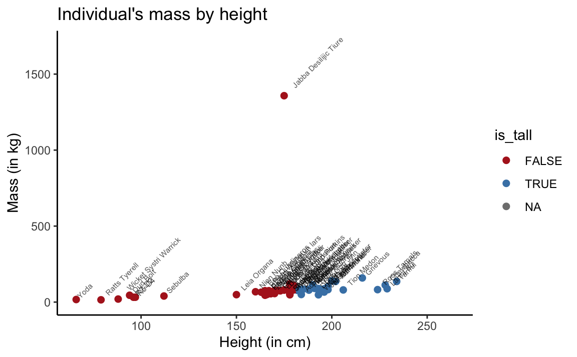

Figure 3.4: Scatterplot of mass by height in the full sw dataset.

Note that we used coord_cartesian to restrict the range of y values shown to ylim = c(0, 1700).

The scatterplot shows that the sw data contains a blatant outlier: Jabba Desilijic Tiure, the crime lord aka. ‘Jabba the Hutt’, has a mass of 1358 kg despite his below-average height of 175 cm. Only considering creatures with a mass up to 170 kg suggests that Yoda’s hypothesis is perfectly valid when this outlier is excluded:

# Only showing mass values from 0 to 180: 
ggplot(sw_tall, aes(x = height, y = mass)) + 
  geom_abline(aes(intercept = lm(mass ~ height)$coefficients[1], slope = lm(mass ~ height)$coefficients[2]), 
              linetype = 2, col = "orange") + 
  # stat_ellipse(aes(color = is_tall), alpha = .5) + 
  geom_point(aes(color = is_tall), size = 2) + 
  geom_text(aes(label = name), hjust = -.2, angle = 45, size = 2, alpha = 2/3) + 
  coord_cartesian(ylim = c(0, 170)) +
  scale_color_manual(values = c("firebrick", "steelblue", "gold")) +
  labs(title = "Individual's mass by height without outlier",
       x = "Height (in cm)", y = "Mass (in kg)") + 
  theme_classic()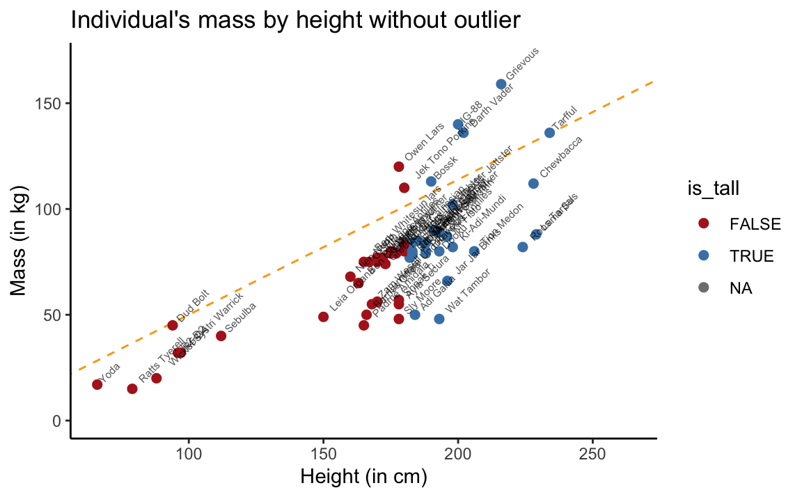

Figure 3.5: Scatterplot of mass by height without Jabba the Hutt.

This is yet another instance of the lesson taught by Anscombe’s quartet (in Section 2.1): We should never interpret the results of some statistical calculation without properly inspecting the underlying data.

References

Bache, S. M., & Wickham, H. (2022). magrittr: A forward-pipe operator for R. Retrieved from https://magrittr.tidyverse.org

Wickham, H., François, R., Henry, L., Müller, K., & Vaughan, D. (2023). dplyr: A grammar of data manipulation. Retrieved from https://dplyr.tidyverse.org