5.2 Essential tibble commands
Whenever working with rectangular data structures — data consisting of multiple cases (rows) and variables (columns) — our first step (in a tidyverse context) is to create or transform the data into a tibble.
A tibble is a rectangular data table and a modern and simpler version of the data.frame construct in R.
As the tibble package (Müller & Wickham, 2026) is part of the core tidyverse, we can load it as follows:
As a preview, Figure 5.2 provides a schematic overview of the roles of the tidyverse packages tibble (discussed in this chapter) and readr (discussed in Chapter 6 on Importing data) for creating tibbles: Both packages provide tools for creating tibbles, but differ in their input sources. Existing tibbles can be used for data analysis (e.g., for data transformations, visualizations, or statistics) or can be written to files (e.g., to be archived or shared).
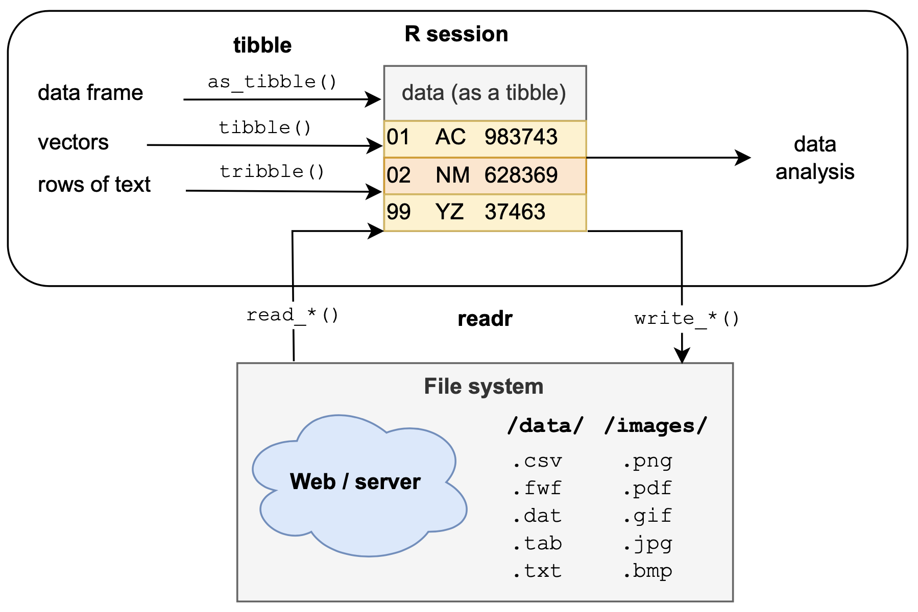
Figure 5.2: The readr and tibble packages use different inputs to create a tabular data structure known as a tibble, which is a simpler data frame. Tibbles can then be used for data analysis in R (e.g., for data transformation, visualization, or statistics) or written to a file (e.g., for archival or sharing purposes).
Tibbles vs. data frames
Whereas data frames appeared in base R in the 1990s (and are a legacy of the S programming language on which R is based), tibbles first appeared in the dplyr package and in the form of an R tibble package (v1.0) in 2016. Nevertheless, tibbles essentially are simpler data frames. In contrast to the base R behavior of data frames, turning data into tibbles is more restrictive. Specifically,
tibbles do not change the types of input variables (e.g., strings are not converted to factors);
tibbles do not change the names of input variables and do not use row names.
While the default behavior of tibbles is more restrictive, tibbles are still flexible, e.g., by also allowing for non-syntactic variable (column) names. For instance, in contrast to data frames, the variable names in tibbles can start with a number or contain space characters:
tb <- tibble(
  `1 age` = c(17, 33, 28, 23, 15),
  ` sex` = c("m", "f", "f", "m", "?")
)
tb
#> # A tibble: 5 × 2
#>   `1 age` ` sex`
#>     <dbl> <chr>
#> 1      17 m
#> 2      33 f
#> 3      28 f
#> 4      23 m
#> 5      15 ?
To refer to names with such unorthodox spellings, they need to be enclosed in backticks ` `.42 But variable names in backticks quickly get cumbersome, for instance:
# Refer to non-syntactic names:
tb$`1 age`
#> [1] 17 33 28 23 15
tb$` sex`[2]
#> [1] "f"

# Transforming data:
tb %>%
  filter(`1 age` > 17) %>%
  arrange(`1 age`)
#> # A tibble: 3 × 2
#>   `1 age` ` sex`
#>     <dbl> <chr>
#> 1      23 m
#> 2      28 f
#> 3      33 f
The precise differences between tibbles and data frames are not important to us at this point.
(The main differences concern printing, subsetting, and the recycling behavior of vector elements when creating tibbles. See vignette("tibble") for details.)
For our present purposes, tibbles are preferable to data frames, as they are easier to understand, easier to manipulate, and thus reduce the chance of problems or unpleasant surprises.
Creating tibbles
The question How can we create tibbles? is more relevant to our concerns. This chapter covers three ways of creating tibbles:
as_tibble()converts (or “coerces”) an existing rectangle of data (e.g., a data frame) into a tibble.tibble()converts several vectors into (the columns of) a tibble.tribble()converts a table (entered row-by-row) into a tibble.
We will illustrate each of these commands in the following sections.
Practice
Before we start creating tibbles, inspect the 3-item list of commands more closely.
The three commands yield the same type of output (i.e., a data table of the tibble variety), but require different inputs.
- Which kind of input(s) does each command expect and how do these inputs need to be structured and formatted (e.g., do they contain parentheses, commas, etc.)?
5.2.1 as_tibble() (from rectangles)
We use the as_tibble() function to create a tibble from data that already is in rectangular format (e.g., a data frame or matrix).
- Starting from a data frame:
## Using the data frame `sleep`: ------
# ?datasets::sleep # provides background information on the data set.
df <- datasets::sleep  # copy

# Convert df into a tibble (tb):
tb <- as_tibble(df)
As always, we can apply some standard functions for inspecting df and tb:
# Inspect the data frame df: ----
dim(df)
#> [1] 20  3
is.data.frame(df)
#> [1] TRUE
head(df)
#>   extra group ID
#> 1   0.7     1  1
#> 2  -1.6     1  2
#> 3  -0.2     1  3
#> 4  -1.2     1  4
#> 5  -0.1     1  5
#> 6   3.4     1  6
str(df)
#> 'data.frame':    20 obs. of  3 variables:
#>  $ extra: num  0.7 -1.6 -0.2 -1.2 -0.1 3.4 3.7 0.8 0 2 ...
#>  $ group: Factor w/ 2 levels "1","2": 1 1 1 1 1 1 1 1 1 1 ...
#>  $ ID   : Factor w/ 10 levels "1","2","3","4",..: 1 2 3 4 5 6 7 8 9 10 ...
As tibbles are data frames, we can use the same commands on tb:
# Inspect the tibble tb: ----
dim(tb)
#> [1] 20  3
is.data.frame(tb)  # => tibbles ARE data frames.
#> [1] TRUE
head(tb)
#> # A tibble: 6 × 3
#>   extra group ID
#>   <dbl> <fct> <fct>
#> 1   0.7 1     1
#> 2  -1.6 1     2
#> 3  -0.2 1     3
#> 4  -1.2 1     4
#> 5  -0.1 1     5
#> 6   3.4 1     6
str(tb)
#> tibble [20 × 3] (S3: tbl_df/tbl/data.frame)
#>  $ extra: num [1:20] 0.7 -1.6 -0.2 -1.2 -0.1 3.4 3.7 0.8 0 2 ...
#>  $ group: Factor w/ 2 levels "1","2": 1 1 1 1 1 1 1 1 1 1 ...
#>  $ ID   : Factor w/ 10 levels "1","2","3","4",..: 1 2 3 4 5 6 7 8 9 10 ...
However, when using tibble, we can use some additional commands:
is.tibble(tb)
#> [1] TRUE
glimpse(tb)
#> Rows: 20
#> Columns: 3
#> $ extra <dbl> 0.7, -1.6, -0.2, -1.2, -0.1, 3.4, 3.7, 0.8, 0.0, 2.0, 1.9, 0.8, …
#> $ group <fct> 1, 1, 1, 1, 1, 1, 1, 1, 1, 1, 2, 2, 2, 2, 2, 2, 2, 2, 2, 2
#> $ ID    <fct> 1, 2, 3, 4, 5, 6, 7, 8, 9, 10, 1, 2, 3, 4, 5, 6, 7, 8, 9, 10
The most obvious advantage of a tibble is that it can simply be printed to see the most important information about a table of data: Its dimensions, types of variables (columns), and the values of the first rows:
tb
#> # A tibble: 20 × 3
#>    extra group ID
#>    <dbl> <fct> <fct>
#>  1   0.7 1     1
#>  2  -1.6 1     2
#>  3  -0.2 1     3
#>  4  -1.2 1     4
#>  5  -0.1 1     5
#>  6   3.4 1     6
#>  7   3.7 1     7
#>  8   0.8 1     8
#>  9   0   1     9
#> 10   2   1     10
#> 11   1.9 2     1
#> 12   0.8 2     2
#> 13   1.1 2     3
#> 14   0.1 2     4
#> 15  -0.1 2     5
#> 16   4.4 2     6
#> 17   5.5 2     7
#> 18   1.6 2     8
#> 19   4.6 2     9
#> 20 3.4 2 10- Starting from an existing matrix:
# create a 5 x 4 matrix of random numbers:
mx <- matrix(rnorm(n = 20, mean = 100, sd = 10), nrow = 5, ncol = 4)
mx
#>           [,1]      [,2]      [,3]      [,4]
#> [1,] 118.95193  93.60005 105.04955 100.36123
#> [2,]  95.69531 104.55450  82.82991 102.05999
#> [3,]  97.42731 107.04837  92.15541  96.38943
#> [4,]  82.36837 110.35104  91.49092 107.58163
#> [5,] 104.60097  93.91074  75.85792  92.73295
As matrices are rectangular data structures, coercing a matrix into a tibble also works with the as_tibble command:
tx <- as_tibble(mx)
tx
#> # A tibble: 5 × 4
#>      V1    V2    V3    V4
#>   <dbl> <dbl> <dbl> <dbl>
#> 1 119.   93.6 105.  100.
#> 2  95.7 105.   82.8 102.
#> 3  97.4 107.   92.2  96.4
#> 4  82.4 110.   91.5 108.
#> 5 105.   93.9  75.9  92.7
Note that — whereas the matrix mx contained no column names — the corresponding tibble tx contains default variable names:
Practice
Convert some other R datasets (e.g.,
datasets::attitude,datasets::mtcars, anddatasets::Orange) into tibbles and inspect their dimensions and contents.- What types of variables (columns of data) do they contain?
- What is their basic unit of observation (i.e., a row of data)?
- What types of variables (columns of data) do they contain?
- Obtain the same information that you get by printing a tibble
tb(i.e., its dimensions, types of variables, and values of the first rows) about some data framedf. How many R functions do you need?
# data:
df <- datasets::mtcars
tb <- as_tibble(df)

tb  # print tibble

dim(df)  # provides dimensions
str(df)  # provides types of variables
df       # provides variables and values
For relatively small data tables, using one versus several short commands may seem comparable. But for larger data sets, using tibbles is much more convenient.43
5.2.2 tibble() (from columns/vectors)
How can we create a tibble when we do not yet have a rectangular data structure? A common case of this type is that we have several vectors (i.e., linear data structures) and want to combine them into a tibble (i.e., tabular data structure). Importantly, the vectors will become the variables (columns) of our tibble.
We use the tibble() function when the data to be turned into a tibble appears as a collection of vectors.
Thus, tibble() is the tibble function that corresponds to data.frame() in base R.
For instance, imagine we want to create a tibble that stores the following information about a family:
| id | name | age | gender | drives | married_2 |
|---|---|---|---|---|---|
| 1 | Adam | 46 | male | TRUE | Eva |
| 2 | Eva | 48 | female | TRUE | Adam |
| 3 | Xaxi | 21 | female | FALSE | Zenon |
| 4 | Yota | 19 | female | TRUE | NA |
| 5 | Zack | 17 | male | FALSE | NA |
One way of viewing this table is as a series of variables that are the columns of the table (rather than its rows). Each column consists of a variable name and the same number of (here: 5) values, which can be of different types (here: numbers, characters, or Boolean truth values). Each column may or may not contain missing values (entered as NA).
The tibble() function expects that each column of the table is entered as a vector:
# Create a tibble from vectors (column-by-column):
fm <- tibble(
  id        = c(1, 2, 3, 4, 5), # OR: id = 1:5,
  name      = c("Adam", "Eva", "Xaxi", "Yota", "Zack"),
  age       = c(46, 48, 21, 19, 17),
  'self-described gender' = c("male", rep("female", 3), "male"),
  drives    = c(TRUE, TRUE, FALSE, TRUE, FALSE),
  married_2 = c("Eva", "Adam", "Zenon", NA, NA)
)

fm  # prints the tibble:
#> # A tibble: 5 × 6
#>      id name    age `self-described gender` drives married_2
#>   <dbl> <chr> <dbl> <chr>                   <lgl>  <chr>
#> 1     1 Adam     46 male                    TRUE   Eva
#> 2     2 Eva      48 female                  TRUE   Adam
#> 3     3 Xaxi     21 female                  FALSE  Zenon
#> 4     4 Yota     19 female                  TRUE   <NA>
#> 5     5 Zack     17 male                    FALSE  <NA>
Note some details on using the tibble() function:
Each vector is labeled by the variable (column) name, which is not quoted (enclosed in quotation marks);
We avoid spaces within variable (column) names (or else enclose names in backticks if we really
must use spaces);Consecutive vectors are separated by commas (but there is no comma after the final vector).
A general feature of R is that any vector is of a single data type (character, logical, numeric, or a factor of categorical values). However, note also that all vectors combined into the tibble fm had the same shape (i.e., length). This begs the question:
- What happens when the to-be-combined vectors are of different lengths?
Let’s try and find out:
# Data (as vectors of different length):
nr       <- 1:2
initials <- c("A.B", "N.N.", "U.N.", "X.Y.")
adult    <- TRUE

# Create a data frame:
data.frame(n = nr,
           i = initials,
           a = adult)
#>   n    i    a
#> 1 1  A.B TRUE
#> 2 2 N.N. TRUE
#> 3 1 U.N. TRUE
#> 4 2 X.Y. TRUE

# Create a tibble:
tibble(n = nr,
       i = initials,
       a = adult)
#> Error in `tibble()`:
#> ! Tibble columns must have compatible sizes.
#> • Size 2: Existing data.
#> • Size 4: Column `i`.
#> ℹ Only values of size one are recycled.
This example illustrates a difference in the default behavior of data.frame() and tibble():
Whereas data.frame() recycles its vectors to the length of the longest vector (as long as the length of the longest vector is a multiple of all shorter vectors), tibble() only recycles vectors of length 1 (i.e., scalars). (Removing the line n = nr from the example would work without a warning, as the logical scalar adult would be recycled to the length of initials.)
A neat feature when using tibble() for creating tibbles is that later vectors may use the values of earlier vectors:
# Using earlier vectors when defining later ones:
abc <- tibble(
  n    = 1:5,
  ltr  = letters[n],
  l_n  = paste(ltr, n, sep = "_"),  # combine ltr with n
  n_sq = n^2                        # square n
  )

abc  # prints the tibble:
#> # A tibble: 5 × 4
#>       n ltr   l_n    n_sq
#>   <int> <chr> <chr> <dbl>
#> 1     1 a     a_1       1
#> 2     2 b     b_2       4
#> 3     3 c     c_3       9
#> 4     4 d     d_4      16
#> 5     5 e     e_5      25
Overall, using tibble() on a collection of vectors is an easy and robust way for creating tibbles.
Practice
Use
tibble()to enter some information on your family (e.g., thename,age, and other features of a few family members) as a tibble.Find some tabular data online (e.g., on Wikipedia) and enter it as a tibble by applying
tibble()to a list of vectors.
5.2.3 tribble() (from rows)
As the third member of key tibble tools, the tribble() function comes into play when the data to be used appears as a collection of rows (or is already in tabular form).
As most datasets use rows for representing their units of observations (e.g., individual cars, people, penguins, etc.), entering them in this fashion often seems natural and straightforward.
For instance, when copying and pasting the above family data from an electronic document, it is easy to insert commas between consecutive cell values and use tribble() for entering each person (row-by-row) into a tibble:
## Create a tibble from tabular data (row-by-row):
fm2 <- tribble(
  ~id, ~name, ~age, ~gender, ~drives,  ~married_2,
  #--|------|-----|--------|----------|----------|
  1,  "Adam", 46,  "male",    TRUE,     "Eva",
  2,  "Eva",  48,  "female",  TRUE,     "Adam",
  3,  "Xaxi", 21,  "female",  FALSE,    "Zenon",
  4,  "Yota", 19,  "female",  TRUE,      NA,
  5,  "Zack", 17,  "male",    FALSE,     NA      )

fm2  # prints the tibble:
#> # A tibble: 5 × 6
#>      id name    age gender drives married_2
#>   <dbl> <chr> <dbl> <chr>  <lgl>  <chr>
#> 1     1 Adam     46 male   TRUE   Eva
#> 2     2 Eva      48 female TRUE   Adam
#> 3     3 Xaxi     21 female FALSE  Zenon
#> 4     4 Yota     19 female TRUE   <NA>
#> 5     5 Zack     17 male   FALSE  <NA>
Note some details on using the tribble() function:
The column names are preceded by the tilde symbol
~and become the variable names of the tibble;Non-standard variable names are quoted (but should be avoided whenever possible);
Consecutive entries are separated by a comma, but there is no comma after the final entry;
The spacing within each row is optional (we chose to add extra spaces and align columns for clarity);
The line
#--|-----|-----|-----|--------|--------|is commented out and can be omitted;The type of each column is determined by the type of the corresponding cell values. For instance, the NA values in
fm2are missing character values because the entries above were characters (entered in quotes).
Check
If tibble() and tribble() really are alternative commands, then the contents of our objects fm and fm2 should be identical:
Practice
Describle the difference between
tibble()andtribble()in your own words.Enter the tibble
abc(from above) by using thetribble()function.Find some tabular data online (e.g., on Wikipedia) and enter it as a tibble by applying
tribble()to rows of data.
This concludes our introduction of the three key tibble creation functions.
However, note that there are important other ways of obtaining tibbles.
Whenever we use functions from tidyverse packages that create rectangular tables, their outputs will probably be tibbles.
For instance, when using functions from the dplyr package (Wickham, François, et al., 2023) to transform and summarize data, they typically yield tibbles (see Chapter 3 on Transforming data).
Similarly, we often obtain tibbles by importing data (e.g., with the read_csv() or read_delim() functions of the readr package, which is covered by the next chapter on Importing data (Chapter 6).
5.2.4 Accessing tibble parts
Once we have a tibble, we typically want to access individual parts of it. Although we already know how rectangular data structures in R can be accessed by indexing (see Section 1.5 and how we can select columns or rows of tibbles by dplyr functions (see Section 3.2), it is helpful to revisit various ways of subsetting tables in the context of tibbles.
We can distinguish between three cases:
- accessing variables (columns),
- accessing cases (rows), and
- accessing values (cells).
1. Accessing variables (columns)
We will select columns from the family tibble fm (defined above):
fm
#> # A tibble: 5 × 6
#>      id name    age gender drives married_2
#>   <dbl> <chr> <dbl> <chr>  <lgl>  <chr>
#> 1     1 Adam     46 male   TRUE   Eva
#> 2     2 Eva      48 female TRUE   Adam
#> 3     3 Xaxi     21 female FALSE  Zenon
#> 4     4 Yota     19 female TRUE   <NA>
#> 5     5 Zack     17 male   FALSE  <NA>
As each column of a tibble is a vector, obtaining a column of the tibble amounts to obtaining the corresponding vector. We can access this vector by its name (label) or by its number (column position):
# Get the name column of fm (as a vector):
fm$name       # by label (with $)
#> [1] "Adam" "Eva"  "Xaxi" "Yota" "Zack"
fm[["name"]]  # by label (with [])
#> [1] "Adam" "Eva"  "Xaxi" "Yota" "Zack"
fm[[2]]       # by number (with [])
#> [1] "Adam" "Eva"  "Xaxi" "Yota" "Zack"
Actually, we know even more ways of obtaining the name information from fm.
However, note that the following commands — which use either base R indexing or dplyr commands — all return a tibble, rather than a vector:
# Get the name column of fm (as a 5 x 1 tibble):
fm[ , 2]
#> # A tibble: 5 × 1
#>   name
#>   <chr>
#> 1 Adam
#> 2 Eva
#> 3 Xaxi
#> 4 Yota
#> 5 Zack
select(fm, 2)
#> # A tibble: 5 × 1
#>   name
#>   <chr>
#> 1 Adam
#> 2 Eva
#> 3 Xaxi
#> 4 Yota
#> 5 Zack
select(fm, name)
#> # A tibble: 5 × 1
#>   name
#>   <chr>
#> 1 Adam
#> 2 Eva
#> 3 Xaxi
#> 4 Yota
#> 5 Zack
Practice
- Use analog commands to obtain the
ageinformation offmeither as a vector or a tibble.
# Get the age column of fm (as a vector):
fm$age        # by name (with $)
fm[["age"]]   # by name (with [])
fm[[3]]       # by number (with [])

# Get the age column of fm (as a 5 x 1 tibble):
fm[ , 3]
select(fm, 3)
select(fm, age)- Extract the
pricecolumn ofggplot2::diamondsin at least 3 different ways and verify that they all yield the same mean price.
2. Accessing cases (rows)
Extracting specific rows of a tibble amounts to filtering a tibble and typically yields smaller tibbles (as a row may contain entries of different types). As we are familiar with essential dplyr commands (see Section 3.2), we can achieve this by filtering specific rows of a tibble by dplyr::filter or select specific rows by dplyr::slice. However, it is also possible to specify the desired rows by logical subsetting (i.e., specifying a condition that results in a Boolean value) or by specifying the desired row number (in numeric subsetting).
The following examples illustrate how we can obtain rows from the family tibble fm (defined above):
fm  # family tibble (defined above):
#> # A tibble: 5 × 6
#>      id name    age gender drives married_2
#>   <dbl> <chr> <dbl> <chr>  <lgl>  <chr>
#> 1     1 Adam     46 male   TRUE   Eva
#> 2     2 Eva      48 female TRUE   Adam
#> 3     3 Xaxi     21 female FALSE  Zenon
#> 4     4 Yota     19 female TRUE   <NA>
#> 5     5 Zack     17 male   FALSE  <NA>
The dplyr command filter() selects cases (rows) based on some condition(s).
Thus, it is similar to logical subsetting (i.e., indexing the rows by tests of column variables that evaluate to vectors of TRUE or FALSE):
fm %>% filter(id > 2)
#> # A tibble: 3 × 6
#>      id name    age gender drives married_2
#>   <dbl> <chr> <dbl> <chr>  <lgl>  <chr>
#> 1     3 Xaxi     21 female FALSE  Zenon
#> 2     4 Yota     19 female TRUE   <NA>
#> 3     5 Zack     17 male   FALSE  <NA>
fm %>% filter(age < 18)
#> # A tibble: 1 × 6
#>      id name    age gender drives married_2
#>   <dbl> <chr> <dbl> <chr>  <lgl>  <chr>
#> 1     5 Zack     17 male   FALSE  <NA>
fm %>% filter(drives == TRUE)
#> # A tibble: 3 × 6
#>      id name    age gender drives married_2
#>   <dbl> <chr> <dbl> <chr>  <lgl>  <chr>
#> 1     1 Adam     46 male   TRUE   Eva
#> 2     2 Eva      48 female TRUE   Adam
#> 3     4 Yota     19 female TRUE   <NA>
Here are the same three filters by using logical subsetting:
fm[fm$id > 2, ]
#> # A tibble: 3 × 6
#>      id name    age gender drives married_2
#>   <dbl> <chr> <dbl> <chr>  <lgl>  <chr>
#> 1     3 Xaxi     21 female FALSE  Zenon
#> 2     4 Yota     19 female TRUE   <NA>
#> 3     5 Zack     17 male   FALSE  <NA>
fm[fm$age < 18, ]
#> # A tibble: 1 × 6
#>      id name    age gender drives married_2
#>   <dbl> <chr> <dbl> <chr>  <lgl>  <chr>
#> 1     5 Zack     17 male   FALSE  <NA>
fm[fm$drives == TRUE, ]
#> # A tibble: 3 × 6
#>      id name    age gender drives married_2
#>   <dbl> <chr> <dbl> <chr>  <lgl>  <chr>
#> 1     1 Adam     46 male   TRUE   Eva
#> 2     2 Eva      48 female TRUE   Adam
#> 3     4 Yota     19 female TRUE   <NA>
The dplyr command slice chooses cases (rows) based on their ordinal number.
Thus, it is similar to numeric subsetting (i.e., indexing the rows of a data table):
fm %>% slice(5)     # get row 5
#> # A tibble: 1 × 6
#>      id name    age gender drives married_2
#>   <dbl> <chr> <dbl> <chr>  <lgl>  <chr>
#> 1     5 Zack     17 male   FALSE  <NA>
fm %>% slice(3:5)   # get rows 3 to 5
#> # A tibble: 3 × 6
#>      id name    age gender drives married_2
#>   <dbl> <chr> <dbl> <chr>  <lgl>  <chr>
#> 1     3 Xaxi     21 female FALSE  Zenon
#> 2     4 Yota     19 female TRUE   <NA>
#> 3     5 Zack     17 male   FALSE  <NA>
fm %>% slice(2, 4)  # get rows 2 and 4
#> # A tibble: 2 × 6
#>      id name    age gender drives married_2
#>   <dbl> <chr> <dbl> <chr>  <lgl>  <chr>
#> 1     2 Eva      48 female TRUE   Adam
#> 2     4 Yota     19 female TRUE   <NA>
Here are the same 3 selections by using numeric subsetting:
fm[5, ]        # get row 5
#> # A tibble: 1 × 6
#>      id name    age gender drives married_2
#>   <dbl> <chr> <dbl> <chr>  <lgl>  <chr>
#> 1     5 Zack     17 male   FALSE  <NA>
fm[3:5, ]      # get rows 3 to 5
#> # A tibble: 3 × 6
#>      id name    age gender drives married_2
#>   <dbl> <chr> <dbl> <chr>  <lgl>  <chr>
#> 1     3 Xaxi     21 female FALSE  Zenon
#> 2     4 Yota     19 female TRUE   <NA>
#> 3     5 Zack     17 male   FALSE  <NA>
fm[c(2, 4), ]  # get rows 2 and 4
#> # A tibble: 2 × 6
#>      id name    age gender drives married_2
#>   <dbl> <chr> <dbl> <chr>  <lgl>  <chr>
#> 1     2 Eva      48 female TRUE   Adam
#> 2     4 Yota     19 female TRUE   <NA>
Practice
- Extract all diamonds from
ggplot2::diamondsthat have at least two carat. How many of them are there and what is their average price?
# (1) In several steps:
# Save data ggplot2::diamonds as dm:
dm <- ggplot2::diamonds

# Filter dm by condition:
dm_2 <- filter(dm, carat >= 2)
nrow(dm_2)  # => 2154 rows (cases)

# Compute the mean price of dm_2 (in 3 ways):
mean(dm_2$price)
mean(dm_2[["price"]])
mean(dm_2[[7]])  # => US-$ 14843.66

# (2) In one pipe:
ggplot2::diamonds %>%
  filter(carat >= 2) %>%
  summarise(nr = n(),
            mn_price = mean(price))
3. Accessing values (cells)
Accessing the values of individual tibble cells is relatively rare, but can be achieved by
explicitly providing both row number
rand column numberc(as[r, c]), or byfirst extracting the column (as a vector
v) and then providing the desired row numberr(v[r]).
fm  # family tibble (defined above):
#> # A tibble: 5 × 6
#>      id name    age gender drives married_2
#>   <dbl> <chr> <dbl> <chr>  <lgl>  <chr>
#> 1     1 Adam     46 male   TRUE   Eva
#> 2     2 Eva      48 female TRUE   Adam
#> 3     3 Xaxi     21 female FALSE  Zenon
#> 4     4 Yota     19 female TRUE   <NA>
#> 5     5 Zack     17 male   FALSE  <NA>

# Getting specific cell values:
fm$name[4]  # getting the name of the 4th row
#> [1] "Yota"
fm[4, 2]    # getting the same name by row and column numbers
#> # A tibble: 1 × 1
#>   name
#>   <chr>
#> 1 Yota

# Note: What if we don't know the row number?
which(fm$name == "Yota")  # get the row number that matches the name "Yota"
#> [1] 4
In practice, accessing individual cell values is mostly needed to check for specific cell values and to change or correct erroneous entries by re-assigning them to a different value.
# Checking and changing cell values: ------

# Check: "Who is Xaxi's spouse?" (in 3 different ways):
fm[fm$name == "Xaxi", ]$married_2
#> [1] "Zenon"
fm$married_2[3]
#> [1] "Zenon"
fm[3, 6]
#> # A tibble: 1 × 1
#>   married_2
#>   <chr>
#> 1 Zenon

# Change: "Zenon" is actually "Zeus" (in 3 different ways):
fm[fm$name == "Xaxi", ]$married_2 <- "Zeus"
fm$married_2[3] <- "Zeus"
fm[3, 6] <- "Zeus"

# Check for successful change:
fm
#> # A tibble: 5 × 6
#>      id name    age gender drives married_2
#>   <dbl> <chr> <dbl> <chr>  <lgl>  <chr>
#> 1     1 Adam     46 male   TRUE   Eva
#> 2     2 Eva      48 female TRUE   Adam
#> 3     3 Xaxi     21 female FALSE  Zeus
#> 4     4 Yota     19 female TRUE   <NA>
#> 5     5 Zack     17 male   FALSE  <NA>
By contrast, a relatively common task is to check an entire tibble (e.g., for the existence or count of missing values, or to replace them by some other value):
# Checking for, counting, and changing missing values: ------

fm  # family tibble (defined above):
#> # A tibble: 5 × 6
#>      id name    age gender drives married_2
#>   <dbl> <chr> <dbl> <chr>  <lgl>  <chr>
#> 1     1 Adam     46 male   TRUE   Eva
#> 2     2 Eva      48 female TRUE   Adam
#> 3     3 Xaxi     21 female FALSE  Zeus
#> 4     4 Yota     19 female TRUE   <NA>
#> 5     5 Zack     17 male   FALSE  <NA>

# (a) Check for missing values:
is.na(fm)       # checks each cell value for being NA
#>         id  name   age gender drives married_2
#> [1,] FALSE FALSE FALSE  FALSE  FALSE     FALSE
#> [2,] FALSE FALSE FALSE  FALSE  FALSE     FALSE
#> [3,] FALSE FALSE FALSE  FALSE  FALSE     FALSE
#> [4,] FALSE FALSE FALSE  FALSE  FALSE      TRUE
#> [5,] FALSE FALSE FALSE  FALSE  FALSE      TRUE

# (b) Count the number of missing values:
sum(is.na(fm))  # counts missing values (by adding up all TRUE values)
#> [1] 2

# (c) Change all missing values:
fm[is.na(fm)] <- "A MISSING value!"

# Check for successful change:
fm
#> # A tibble: 5 × 6
#>      id name    age gender drives married_2
#>   <dbl> <chr> <dbl> <chr>  <lgl>  <chr>
#> 1     1 Adam     46 male   TRUE   Eva
#> 2     2 Eva      48 female TRUE   Adam
#> 3     3 Xaxi     21 female FALSE  Zeus
#> 4     4 Yota     19 female TRUE   A MISSING value!
#> 5 5 Zack 17 male FALSE A MISSING value!5.2.5 From tibbles to data frames
As any tibble also is (a special type of) data frame, we rarely need to convert a tibble tb into a data frame.
However, some R functions require an original data frame — mostly because they expect tb[ , i] to return the \(i\)-th column of tb as a vector, when it actually will return another tibble:
# Using the tibble fm (from above):
class(fm)  # tibbles are a kind of data.frame
#> [1] "tbl_df"     "tbl"        "data.frame"
fm[ , 2]   # yields the 2nd column as a tibble (!)
#> # A tibble: 5 × 1
#>   name
#>   <chr>
#> 1 Adam
#> 2 Eva
#> 3 Xaxi
#> 4 Yota
#> 5 Zack
fm[[2]]    # yields the 2nd column as a vector
#> [1] "Adam" "Eva"  "Xaxi" "Yota" "Zack"
For rare cases like this, it is good to know that R has a as.data.frame() function
that always allows turning a tibble into a data frame:
# Turn the tibble fm into a data frame:
df_fm <- as.data.frame(fm)

class(df_fm)  # an ordinary data.frame
#> [1] "data.frame"
df_fm[ , 2]   # yields the 2nd column as a vector (!)
#> [1] "Adam" "Eva"  "Xaxi" "Yota" "Zack"
df_fm[[2]]    # yields the 2nd column as a vector
#> [1] "Adam" "Eva"  "Xaxi" "Yota" "Zack"
5.2.6 Conclusion
Our focus in this section was on creating tibbles and accessing parts of tibbles. Prior to this chapter, we were already working with tibbles, but encountered them mostly as data objects provided by packages, inputs of ggplot2 functions, and outputs of dplyr pipes. More advanced transformations of tibbles were discussed in the context of on Transforming data (Chapter 3). The following chapters will continue to use tibbles and teach us new ways of importing (Chapter 6) and combining (Chapter 8) tibbles, or wrangling them into various shapes (Chapter 7).
At this point, it may seem as if tibbles are the only data structure that we will ever need. This impression is wrong, but has a simple reason: In this book, we focus on rectangular data that can conveniently be stored as a tibble. Although it is impressive how many things can be expressed in this format, tibbles are just a convenient way of starting our expedition into data science. Clearly, there are lots of types of information that are of immense scientific interest, but not easily stored in this format — for instance images, texts, sounds, tastes, and most natural phenomena (e.g., psychological, economic, or social processes).