14 Tidying data

Transforming data generally turns data structures into other data structures. Whereas Chapter 13 taught us to use pipes of dplyr functions, this chapter continues our journey into data transformation by adding tidyr functions.

Theoretically, we distinguished between reshaping and reducing data (see Section 13.1.2). Whereas the dplyr pipes of Chapter 13 were mostly used to reshape and reduce data for answering data-based questions (e.g., by summarizing over the levels of a variable), our main focus in the present chapter on tidyr will be on reshaping data into a form that can easily be processed and understood.

The key concepts and topics of this chapter are:

Section 14.2.1 discusses the notions of “messy” and “tidy” data
Section 14.2.2 explains how to transform data tables with tools from the tidyr package (Wickham & Girlich, 2024)

Although transforming data can be viewed as a challenge and a task in itself, our primary goal usually consists in gaining insights into the contents of our data. From this perspective, transforming data (by reshaping or reducing it) becomes an intermediate goal, or a means to an end — a way of representing our data so that it can be processed faster and better understood.

Preparation

Recommended readings for this chapter include

Chapter 7: Tidying data of the ds4psy book (Neth, 2023a)
Chapter 12: Tidy data of the r4ds book (Wickham & Grolemund, 2017)

Preflections

Before reading, please take some time to reflect upon the following questions:

Does it matter in what shape data is stored? Why or why not?
If two datasets contain the same data, how could one structure be superior to another?
What could be considered “messy” data? What would be required to “tidy” it?

14.1 Introduction

We previously distinguished between data transformations that reduce and reshape data (in Section 13.1 of Chapter 13). Reducing data usually goes beyond mere “trans-formation” by being uni-directional: We typically cannot reconstruct the original data from reduced data. By contrast, reshaping operations can be reversed, in the sense that the original and the reshaped data contain the same information. But this raises the question:

Why is reshaping data needed or useful at all?

Our answer to this question alludes to a famous quote of George Orwell’s Animal Farm:

All reshaped data structures are equal, but some are more equal than others.

Without additional explanations, this may only seem to muddy our explanation further. For in what sense can some data structure be superior to another, when they merely differ in shape? Before we address the issue of some forms being better or worse than others, we need to understand how different forms can contain the same data. The following examples will help to illuminate this issue.

14.1.1 Reflection: Same or different data?

Suppose we were interested in the number of tuberculosis (TB) cases documented by the World Health Organization of three countries (e.g., Afghanistan, Brazil, and China) and two years (e.g., 1999 and 2000).

Our first insight should be that absolute numbers of cases are good to know, but difficult to interpret by themselves. Given that China is much larger than Afghanistan, we should expect higher numbers for most diseases that can occur in either country. Thus, we should also know each country’s population to put the number of cases into perspective. Thus, our data contains 2 variables (TB cases and population) for 3 countries and 2 different time points (i.e., a total of $2 \cdot 3 \cdot 2 = 12$ numeric data points).

Suppose we had these 12 numbers — but how would we organize them into a table? A second insight is that there are many different ways in which we could present the same data. Compare and contrast the following data tables:

#> [1] 6 4

Table 14.1: The data of `tidyr::table1`.
country	year	cases	population
Afghanistan	1999	745	19987071
Afghanistan	2000	2666	20595360
Brazil	1999	37737	172006362
Brazil	2000	80488	174504898
China	1999	212258	1272915272
China	2000	213766	1280428583

#> [1] 12  4

Table 14.2: The data of `tidyr::table2`.
country	year	type	count
Afghanistan	1999	cases	745
Afghanistan	1999	population	19987071
Afghanistan	2000	cases	2666
Afghanistan	2000	population	20595360
Brazil	1999	cases	37737
Brazil	1999	population	172006362
Brazil	2000	cases	80488
Brazil	2000	population	174504898
China	1999	cases	212258
China	1999	population	1272915272
China	2000	cases	213766
China	2000	population	1280428583

#> [1] 6 1

Table 14.3: The data of `ds4psy::table7`.
where_when_what
Afghanistan@19:99$745\19987071
Afghanistan@20:00$2666\20595360
Brazil@19:99$37737\172006362
Brazil@20:00$80488\174504898
China@19:99$212258\1272915272
China@20:00$213766\1280428583

#> [1] 3 5

Table 14.4: The data of `ds4psy::table8`.
country	cases_1999	cases_2000	popu_1999	popu_2000
Afghanistan	745	2666	19987071	20595360
Brazil	37737	80488	172006362	174504898
China	212258	213766	1272915272	1280428583

Before reading on, let’s compare the tables and answer the following questions:

In which sense are these tables different? (Note their dimensions, variables, etc.)
In which sense do all these tables represent the same data?
Is any of the tables better or worse than the others?

The data contains values associated with four variables (e.g., country, year, cases, and population), but each table organizes the values in a different layout. Describing these layouts reports varying number of rows and columns (i.e., vectors or tables of different shapes) and perhaps terms like implicit or explicit. Importantly, the tables are all identical — or informationally equivalent — in the sense that they can be transformed into each other without gaining or losing information.

Which actions or operations would we need to perform to transform any table into one of the others? By the end of this chapter, we can do all this by using the tools provided by dplyr and tidyr. In addition, we will have acquired some new terminology for describing tables (using labels like “longer” or “wider”, or “messy” or “tidy”) and a pipe operator that allows creating chains of commands.

14.1.2 Key concepts

In addition to introducing the tidyverse package tidyr, this chapter adds more terminology for talking about data transformations:

Section 14.2.1 introduces concepts to distinguish “tidy” from “messy” data.
Section 14.2.2 on transforming tables with tidyr introduce tools for tidying data. These imply additional terminology and functions to unite or separate and gather or spread variables. In the database lingo of related contexts, reshaping tables is also known as folding and unfolding variables, melting or casting columns, or pivoting tables into longer or wider formats.

What data structures are being reshaped? As in the previous chapter, we still mostly transform tables into other tables. Thus, the pipe operator %>% from the magrittr package (Bache & Wickham, 2022) is still useful and the reshaping functions of tidyr can be combined flexibly with the reducing or reshaping functions of dplyr.

Given that dplyr and tidyr seem so similar, another question to ask in this chapter is: What is the difference between transforming data with dplyr and with tidyr? We will address this question after introducing the essential tidyr functions (in Section 14.3.1).

14.2 Transforming data with tidyr

Tidy datasets are all alike
but every messy dataset is messy in its own way.

Hadley Wickham (2014b, p. 2)

This quote by Hadley Wickham is a variation of the initial sentence of Tolstoy’s novel Anna Karenina. In both version, it is implied that all entities (i.e., happy families or tidy datasets) share some characteristic feature, whereas there is a variety of ways in which things can go wrong (i.e., become unhappy or messy). Both sentences convey great insights, of course, but explaining why they are true is a bit like explaining a joke — and not quite as catchy.

The term “tidy data” comes from the related concept of “data cleaning”. Cleaning up data can be a boring and laborious phase of data analysis, but is also decisive for obtaining meaningful results. The “tidy data” concept was defined in contrast to “messy data” (e.g., by Wickham, 2014b) and is the eponym for the tidyverse and the tidyr package.

The following sections merely provide a summary of essential tidyr functions. More extensive resources for this section include:

Chapter 7: Tidying data of the ds4psy book (Neth, 2023a).
Chapter 12: Tidy data of the r4ds book (Wickham & Grolemund, 2017).
The documentation of the tidyr package (Wickham & Girlich, 2024).

14.2.1 What is tidy data?

What is tidy data? The notion of tidy data is a key inspiration for the tidyverse. The concept of “tidy” is neat and intuitive, but also a bit vague. Rather than attempting a formal definition, we will characterize the term by describing the intentions behind its uses:

Informally, tidy data serves as the antagonist of messy data. As messy data is data that is difficult to work with, data is considered “tidy” when it is easy to work with.
The key idea of tidy data is that each variable should be in its own column.

Both these descriptions sound rather trivial, of course. The second point raises the question: When is a variable not in its own column?

The trick here is that the term “variable” is used in a functional sense: A variable is some measure or description that we want to use as a variable in an analysis. For instance, depending on the particular task at hand, a “variable” could be a particular date, or the month, year, or century that corresponds to a date. Thus, what is considered to be “tidy” partly lies in the eyes of the beholder and depends on what someone wants to do with data, rather than on some inherent property of the data itself.

More generally, the notion of tidy data is illuminated within a framework of ecological rationality (see Section 1.2.5): The difference between messy and tidy data depends on (a) our goals or the intended use of the data (e.g., which task do we want to address?) and (b) the tools with which we typically carry out our tasks (e.g., which functions are we familiar with?). Given the tools provided by R and prominent R packages (e.g., dplyr or ggplot2), it makes sense to first identify the variables of our analysis and then reshape the data so that each variable is in its own column. Although this format is informationally equivalent to many alternative formats, it provides practical benefits for further transforming the data. For instance, we can use the variables to filter, select, group, or pivot the data to reshape or reduce it to answer our questions.

14.2.2 Essential tidyr functions

The tidyr package (Wickham & Girlich, 2024) provides commands to create and transform messy into tidy data (or vice versa). Although the package provides many functions, we consider two pairs of two complementary tidyr commands as essential:

separate() splits one variable into two variables;
unite() combines two variables into one variable;
pivot_longer() or gather() make (“wide”) data longer (by gathering many variables into one variable);
pivot_wider() or spread() make (“long”) data wider (by spreading one variable into many variables).

The first two commands allow splitting or combining variables: separate() is the complement to or inverse/opposite of unite(). The second two pairs of commands allow changing the data layout by making a given table longer or wider: spread() and pivot_wider() are the complements to or inverses/opposites of gather() and pivot_longer().

In the following sections, we briefly explain how to use these four essential commands.

The table5 tibble of the tidyr package presents two obstacles to tidy data:

table5
#> # A tibble: 6 × 4
#>   country     century year  rate             
#>   <chr>       <chr>   <chr> <chr>            
#> 1 Afghanistan 19      99    745/19987071     
#> 2 Afghanistan 20      00    2666/20595360    
#> 3 Brazil      19      99    37737/172006362  
#> 4 Brazil      20      00    80488/174504898  
#> 5 China       19      99    212258/1272915272
#> 6 China       20      00    213766/1280428583

Instead of solving typical tasks in terms of century and a 2-digit code of year, we normally would encode the year as a 4-digit number. Doing so would require combining two variables into one — which is what the unite() function is for.
The variable rate suffers from the opposite problem: It contains both the number of TB cases and the population count, separated by a forward slash “/”. Splitting one variable into two is the job of the separate() function.

14.2.3 Unite variables

To combine the variables century and year of table5 into a single variable, we can use the following unite() expression:

# Original table:
table5
#> # A tibble: 6 × 4
#>   country     century year  rate             
#>   <chr>       <chr>   <chr> <chr>            
#> 1 Afghanistan 19      99    745/19987071     
#> 2 Afghanistan 20      00    2666/20595360    
#> 3 Brazil      19      99    37737/172006362  
#> 4 Brazil      20      00    80488/174504898  
#> 5 China       19      99    212258/1272915272
#> 6 China       20      00    213766/1280428583

# Unite the "century" & "year" variables into a new column "yr":
table5 %>%
  unite(col = "yr", c("century", "year"), sep = "")
#> # A tibble: 6 × 3
#>   country     yr    rate             
#>   <chr>       <chr> <chr>            
#> 1 Afghanistan 1999  745/19987071     
#> 2 Afghanistan 2000  2666/20595360    
#> 3 Brazil      1999  37737/172006362  
#> 4 Brazil      2000  80488/174504898  
#> 5 China       1999  212258/1272915272
#> 6 China       2000  213766/1280428583

Note that this unite() function is preceded by the pipe operator, so that table5 is used as its first argument (run ?unite to discover its arguments as unite(data, col, ..., sep, remove, na.rm)). Evaluating the pipe creates a 6 x 3 tibble with a new variable yr and removes the two original variables (century and year) from the table, as the remove argument of unite() is set to TRUE by default. Incidentally, omitting the quotation marks around the variable names (here: yr, century, and year) works just as well. Additionally, the new variable yr is of type “character”. To create a corresponding number or factor, we could use mutate() to create additional variables:

table5 %>%
  unite(col = "yr", c("century", "year"), sep = "") %>%
  mutate(yr_num = as.numeric(yr),
         yr_fac = as.factor(yr))

#> # A tibble: 6 × 5
#>   country     yr    rate              yr_num yr_fac
#>   <chr>       <chr> <chr>              <dbl> <fct> 
#> 1 Afghanistan 1999  745/19987071        1999 1999  
#> 2 Afghanistan 2000  2666/20595360       2000 2000  
#> 3 Brazil      1999  37737/172006362     1999 1999  
#> 4 Brazil      2000  80488/174504898     2000 2000  
#> 5 China       1999  212258/1272915272   1999 1999  
#> 6 China       2000  213766/1280428583   2000 2000

or use transmute() to drop yr in favor of an alternative variable.

In case of wondering why we specified sep = "" and whether the order of variables in the expression matters, we can try the following variants:

# with quotes (and sep default):
table5 %>% 
  unite(col = "yr", c("century", "year"))
#> # A tibble: 6 × 3
#>   country     yr    rate             
#>   <chr>       <chr> <chr>            
#> 1 Afghanistan 19_99 745/19987071     
#> 2 Afghanistan 20_00 2666/20595360    
#> 3 Brazil      19_99 37737/172006362  
#> 4 Brazil      20_00 80488/174504898  
#> 5 China       19_99 212258/1272915272
#> 6 China       20_00 213766/1280428583

# without quotes, but different order and sep = "":
table5 %>% 
  unite(col = yr, c(year, century), sep = "")
#> # A tibble: 6 × 3
#>   country     yr    rate             
#>   <chr>       <chr> <chr>            
#> 1 Afghanistan 9919  745/19987071     
#> 2 Afghanistan 0020  2666/20595360    
#> 3 Brazil      9919  37737/172006362  
#> 4 Brazil      0020  80488/174504898  
#> 5 China       9919  212258/1272915272
#> 6 China       0020  213766/1280428583

Thus, sep = "_" by default, and the order of variables matters, but variable names can be quoted or unquoted.

14.2.4 Separate variables

The second issue of table5 involved the rate variable. The separate() function of tidyr allows creating two variables:

# Original table:
table5
#> # A tibble: 6 × 4
#>   country     century year  rate             
#>   <chr>       <chr>   <chr> <chr>            
#> 1 Afghanistan 19      99    745/19987071     
#> 2 Afghanistan 20      00    2666/20595360    
#> 3 Brazil      19      99    37737/172006362  
#> 4 Brazil      20      00    80488/174504898  
#> 5 China       19      99    212258/1272915272
#> 6 China       20      00    213766/1280428583

# Separate the "rate" variable into 2 variables "cases" & "population":
table5 %>%
  separate("rate", into = c("cases", "popu"))
#> # A tibble: 6 × 5
#>   country     century year  cases  popu      
#>   <chr>       <chr>   <chr> <chr>  <chr>     
#> 1 Afghanistan 19      99    745    19987071  
#> 2 Afghanistan 20      00    2666   20595360  
#> 3 Brazil      19      99    37737  172006362 
#> 4 Brazil      20      00    80488  174504898 
#> 5 China       19      99    212258 1272915272
#> 6 China       20      00    213766 1280428583

Note that we did not need to specify sep = "/", as separate() was smart enough to identify this as the only plausible splitting point. If we wanted to separate a variable without a dedicated symbol that signals the separation, we can also specify the numeric position at which we want to split a variable:

# Separate the "country" variable into 2 parts (based on position):
table5 %>%
  separate(country, into = c("ini", "rest"), sep = 3)

#> # A tibble: 6 × 5
#>   ini   rest     century year  rate             
#>   <chr> <chr>    <chr>   <chr> <chr>            
#> 1 Afg   hanistan 19      99    745/19987071     
#> 2 Afg   hanistan 20      00    2666/20595360    
#> 3 Bra   zil      19      99    37737/172006362  
#> 4 Bra   zil      20      00    80488/174504898  
#> 5 Chi   na       19      99    212258/1272915272
#> 6 Chi   na       20      00    213766/1280428583

As the rate and country variables that were separated are no longer part of the resulting tibble, we now have remove = FALSE by default. Finally, the new variables are still of type “character” (i.e., would require a round of “as.numeric()” to be turned into numbers).

14.2.5 Practice: Unite and separate in pipes

Combine the unite() and separate() steps from above in one pipe.

Solution

table5 %>%
  unite(col = yr, c(century, year), sep = "") %>%
  separate(rate, into = c("cases", "popu"))

Note that we may want to mutate some character variables into numeric variables prior to further processing.

Combine the above unite() step (to create the yr variable) with a separate() step that reverses its effect in a single tidyr pipe (to return table5 again).

Solution

table5 %>%
  unite(col = "yr", c("century", "year"), sep = "") %>%
  separate(yr, into = c("century", "year"), sep = 2)

Combine the above separate() step (to split the rate variable into two variables) with a unite() step that reverses its effect in a single tidyr pipe (to return table5 again).

Solution

table5 %>%
  separate(rate, into = c("cases", "popu")) %>%
  unite(col = "rate", c("cases", "popu"), sep = "/")

See Section 7.2 Essential tidyr commands for additional examples and practice tasks.

14.2.6 Making tables longer

When describing the shape of datasets, notions like “wide” and “long” make more sense when describing changes than in absolute terms. For instance, data tables in “wide format” can contain thousands of cases (which most people would consider quite “long”) and tables in “long format” can contain a large number of variables (i.e., be considered quite “wide”). However, the relative terms “longer” and “wider” make sense when describing a change in format of the same data table.

The first change considered here makes a (“wide”) data table (e.g.,, a table in which a single variable is distributed over multiple columns) longer. A simple case for such a task is provided by the data of table4a of the tidyr package:

table4a
#> # A tibble: 3 × 3
#>   country     `1999` `2000`
#>   <chr>        <dbl>  <dbl>
#> 1 Afghanistan    745   2666
#> 2 Brazil       37737  80488
#> 3 China       212258 213766

Using `gather()` for making wide tables longer

Making wide tables longer can be achieved with the gather() command of tidyr. Gathering multiple columns requires that each cell value to be moved is described by a so-called key (e.g., the name of a variable that describes or identifies the value) and its value (e.g., the name of the variable that is being measured). Additionally, we need to specify which variables of a table are to be gathered (by specifying either a vector or range of variables). In the case of table4a, the corresponding gather() command could be:

table4a %>% 
  gather(key = "year", value = "cases", '1999':'2000')

#> # A tibble: 6 × 3
#>   country     year   cases
#>   <chr>       <chr>  <dbl>
#> 1 Afghanistan 1999     745
#> 2 Brazil      1999   37737
#> 3 China       1999  212258
#> 4 Afghanistan 2000    2666
#> 5 Brazil      2000   80488
#> 6 China       2000  213766

Note that the range of to-be-gathered variables (i.e., 1999:2000) lacks an argument name, uses the :-notation to specify a range of variables (but could also be expressed as a two-variable vector c('1999', '2000')), and encloses the variable name in single quotes because the variables '1999' and '2000' start with a number, rather than a letter (as variables in R normally should).

A potential limitation of gather() is that it is primarily designed for cases in which the values of one variable are spread over multiple columns. However, a common case in many datasets is that there are several variables whose values are scattered over multiple columns. For instance, consider the following table8 from the ds4psy package:

ds4psy::table8
#> # A tibble: 3 × 5
#>   country     cases_1999 cases_2000  popu_1999  popu_2000
#>   <chr>            <dbl>      <dbl>      <dbl>      <dbl>
#> 1 Afghanistan        745       2666   19987071   20595360
#> 2 Brazil           37737      80488  172006362  174504898
#> 3 China           212258     213766 1272915272 1280428583

In table8, the contents of table4a are followed by two more columns from table4b, and the meaning of each column (and the variables it contains) is signaled by the column names. One way of reshaping table8 into a longer format would be to split it into two parts (i.e., table4a and table4b), use gather() on each part, and then join the two resulting tables (see the Practice exercises below). An alternative consists in using gather() on all variables with values and later separate() the key variable (containing the previous column names) into two variables:

table8 %>%
  gather(key = "key", value = "nr", cases_1999:popu_2000) %>%
  separate(col = key, into = c("type", "year"))

#> # A tibble: 12 × 4
#>    country     type  year          nr
#>    <chr>       <chr> <chr>      <dbl>
#>  1 Afghanistan cases 1999         745
#>  2 Brazil      cases 1999       37737
#>  3 China       cases 1999      212258
#>  4 Afghanistan cases 2000        2666
#>  5 Brazil      cases 2000       80488
#>  6 China       cases 2000      213766
#>  7 Afghanistan popu  1999    19987071
#>  8 Brazil      popu  1999   172006362
#>  9 China       popu  1999  1272915272
#> 10 Afghanistan popu  2000    20595360
#> 11 Brazil      popu  2000   174504898
#> 12 China       popu  2000  1280428583

However, this only works for table8 because the columns had sensible and systematic column names. A more flexible range of solutions is supported by the pivot_longer() function.

Using `pivot_longer()` rather than `gather()`

In recent versions of tidyr (e.g., version 1.1.0+), the documentation of gather() carries a warning label: “Development on gather() is complete, and for new code we recommend switching to pivot_longer(), which is easier to use, more featureful, and still under active development.” Hence, we can still use gather(), but using the more recent pivot_longer() command is a safer choice. Making table4a wider with this function can be achieved as follows:

table4a %>% 
  pivot_longer(cols = `1999`:`2000`, 
               names_to = "year", values_to = "cases")

#> # A tibble: 6 × 3
#>   country     year   cases
#>   <chr>       <chr>  <dbl>
#> 1 Afghanistan 1999     745
#> 2 Afghanistan 2000    2666
#> 3 Brazil      1999   37737
#> 4 Brazil      2000   80488
#> 5 China       1999  212258
#> 6 China       2000  213766

For simple cases, pivot_longer() works just like gather(): The range of variables (columns) to be changed to a longer format are specified by the cols argument, and the cryptic key and value arguments of gather() are replaced by more intuitive names_to and values_to arguments.

The main benefit of pivot_longer() is that it provides functionalities beyond those of gather(). For instance, the function can gather the two distributed variables of table8 in one expression:

ds4psy::table8 %>%
  pivot_longer(cols = cases_1999:popu_2000, 
               names_to = c("type", "year"), 
               names_sep = "_", 
               # names_pattern = "(.*)_(.*)", 
               values_to = "nr")

#> # A tibble: 12 × 4
#>    country     type  year          nr
#>    <chr>       <chr> <chr>      <dbl>
#>  1 Afghanistan cases 1999         745
#>  2 Afghanistan cases 2000        2666
#>  3 Afghanistan popu  1999    19987071
#>  4 Afghanistan popu  2000    20595360
#>  5 Brazil      cases 1999       37737
#>  6 Brazil      cases 2000       80488
#>  7 Brazil      popu  1999   172006362
#>  8 Brazil      popu  2000   174504898
#>  9 China       cases 1999      212258
#> 10 China       cases 2000      213766
#> 11 China       popu  1999  1272915272
#> 12 China       popu  2000  1280428583

As the names_to argument specifies two variables, we need to say how the column names are to be mapped to the two new variables. This can either be done by specifying a separation marker sep (which can be a character or a numeric value) or by providing a names_pattern (as a regular expression, see Appendix E: Using regular expressions for an introduction).

More advanced features of `pivot_longer()`

The pivot_longer() function allows doing more than gather(), but the price of using its more advanced features is additional complexity within the function. Here are some helpful examples from the documentation of pivot_longer() (see the vignette("pivot") for explanations):

Using the relig_income data:
Using the billboard data:

The tidyr::billboard data provides top-100 song rankings for the year 2000. The data provides variables for the artist name, the track (or song) name, and the date on which a song first appeared in the top-100 ratings (date.enter). After this, a range of variables from wk1 to wk76 notes a track’s rank in each week after it entered. As most songs disappear from the rankings after some weeks, later variables (i.e., columns on the right side of the billbard table) contain an increasing number of missing (or NA) values:

# Data documentation: 
?billboard

# Inspect data:
billboard
glimpse(billboard)

# Note: 
sum(!is.na(billboard))  # existing values
sum(is.na(billboard))   # missing values

The following pivot_longer() command identifies the variables (or cols) to be gathered (or moved from a wide to a longer format) by their common prefix "wk". Specifying names_prefix = "wk" further ensures that the values in the new variable week drop the "wk" prefix (and could thus be transformed into numbers). Finally, the values_drop_na = TRUE argument ensures that the NA values are removed from the resulting tibble:

billboard %>%
 pivot_longer(
   cols = starts_with("wk"),
   names_to = "week",
   names_prefix = "wk",
   values_to = "rank",
   values_drop_na = TRUE)

#> # A tibble: 5,307 × 5
#>    artist  track                   date.entered week   rank
#>    <chr>   <chr>                   <date>       <chr> <dbl>
#>  1 2 Pac   Baby Don't Cry (Keep... 2000-02-26   1        87
#>  2 2 Pac   Baby Don't Cry (Keep... 2000-02-26   2        82
#>  3 2 Pac   Baby Don't Cry (Keep... 2000-02-26   3        72
#>  4 2 Pac   Baby Don't Cry (Keep... 2000-02-26   4        77
#>  5 2 Pac   Baby Don't Cry (Keep... 2000-02-26   5        87
#>  6 2 Pac   Baby Don't Cry (Keep... 2000-02-26   6        94
#>  7 2 Pac   Baby Don't Cry (Keep... 2000-02-26   7        99
#>  8 2Ge+her The Hardest Part Of ... 2000-09-02   1        91
#>  9 2Ge+her The Hardest Part Of ... 2000-09-02   2        87
#> 10 2Ge+her The Hardest Part Of ... 2000-09-02   3        92
#> # ℹ 5,297 more rows

Note that the new week variable is of type “character”, but we could easily turn it into a numeric variable by adding a mutate() step of mutate(nr_wk = as.numeric(week)).

Using the who data:

The tidyr::who data encodes a lot of information (regarding the diagnosis, gender, and age, of the people described in the corresponding frequency counts) in the name of its 56 rightmost variables. To extract this information from the variable names, the names_to argument of pivot_longer() can use multiple names of new variables and the names_pattern argument accepts a regular expression that parses the names according to some pattern:

# Data:
# who
dim(who)

# Multiple variables stored in column names: 
who %>% pivot_longer(
  cols = new_sp_m014:newrel_f65,
  names_to = c("diagnosis", "gender", "age_group"),
  names_pattern = "new_?(.*)_(.)(.*)",
  values_to = "count")

This is nicely illustrates the superior powers of pivot_longer(), but requires some expertise in using regular expressions in R (see Appendix E: Using regular expressions).

Using the anscombe data:

An example only intelligible to expert users is the following (using the anscombe data from the datasets package):

datasets::anscombe

# Multiple observations per row
anscombe %>%
 pivot_longer(everything(),
   names_to = c(".value", "set"),
   names_pattern = "(.)(.)") %>%
  arrange(set)

An explanation of this example, and many others, is available in vignette("pivot"). These examples show that people spend a lot of time and effort on reshaping data files. Our more modest goal here is to understand the basics…

14.2.7 Practice: Making tables longer

The shape of table4b is identical to table4a, but the values represent population counts, rather than counts of cases.

Use both gather() and pivot_longer() to make table4b (containing the countries’ population values) longer:

Solution

table4b

table4b %>% 
  gather(key = "year", value = "population", `1999`:`2000`)

table4b %>% 
  pivot_longer(c(`1999`, `2000`), 
               names_to = "year", values_to = "population")

What would we need to create table1 from the longer versions of the same data in table4a and table4b?

table1
#> # A tibble: 6 × 4
#>   country      year  cases population
#>   <chr>       <dbl>  <dbl>      <dbl>
#> 1 Afghanistan  1999    745   19987071
#> 2 Afghanistan  2000   2666   20595360
#> 3 Brazil       1999  37737  172006362
#> 4 Brazil       2000  80488  174504898
#> 5 China        1999 212258 1272915272
#> 6 China        2000 213766 1280428583

Solution

We could create table1 from table4a and table4b in two steps:

First, we would transform both table4a and table4b from their wide format into a longer format, so that cases and population would be a variable with a single column (as we have just done).
In a second step, we would need to combine both resulting tables: Provided that both outputs in longer formats are arranged the same way, we could add one of the variables (either cases or population) to the other table.

A safer way of combining both tables would join them based on their common variables (e.g., by using the merge() function of base R or one of the join functions of dplyr, see Chapter 8: Joining data of the ds4psy book).

14.2.8 Making tables wider

The opposite of making (“wide”) tables longer is making (“long”) tables wider. And the inverse of gather() in the tidyr package is spread().

Using `spread()` for making long tables wider

The simplest case for the spread() function is that we have a single key variable (whose values are to be turned into new variable names) and a single value variable (whose values are to be distributed over multiple variables). For instance, if we removed the population variable from table1, we could spread the values of the cases variable over two new variables whose names are generated from the year variable (to obtain table4a):

# Select & spread (see table4a):
table1 %>%
  select(-population) %>% 
  spread(key = year, value = cases)

#> # A tibble: 3 × 3
#>   country     `1999` `2000`
#>   <chr>        <dbl>  <dbl>
#> 1 Afghanistan    745   2666
#> 2 Brazil       37737  80488
#> 3 China       212258 213766

Removing the cases variable would allow spreading the remaining values of table1 so that the values of the population variable are spread over two new variables whose names are generated from the year variable (to obtain table4b):

# Select & spread (see table4b):
table1 %>%
  select(-cases) %>% 
  spread(key = year, value = population)

#> # A tibble: 3 × 3
#>   country         `1999`     `2000`
#>   <chr>            <dbl>      <dbl>
#> 1 Afghanistan   19987071   20595360
#> 2 Brazil       172006362  174504898
#> 3 China       1272915272 1280428583

Unfortunately, just like we saw for gather() above, the spread() function is designed for a single dependent variable. However, we often deal with multiple variables (e.g., table1 contains the variables cases and populations, both of which contain frequency counts that we may want to spread into a wider table format. How could we spread multiple variables at once?

Using `pivot_wider()` rather than `spread()`

Perhaps not surprisingly, the more potent replacement of spread() in the tidyr package is called pivot_wider(). To illustrate its potential, we can distinguish between two cases:

Case 1: Our table1 data

table1
#> # A tibble: 6 × 4
#>   country      year  cases population
#>   <chr>       <dbl>  <dbl>      <dbl>
#> 1 Afghanistan  1999    745   19987071
#> 2 Afghanistan  2000   2666   20595360
#> 3 Brazil       1999  37737  172006362
#> 4 Brazil       2000  80488  174504898
#> 5 China        1999 212258 1272915272
#> 6 China        2000 213766 1280428583

can be viewed as containing one independent variable (year) and two dependent variables (cases and population). When reshaping data by spreading it from a (“long”) table into a wider table, the independent variable should provide the names of a new variable and the two dependent variables should become the values of the new variable. The following pivot_wider() expression does this in one step:

# 1. One IV, two DVs: 
table1 %>%
  pivot_wider(names_from = year, 
              values_from = c(cases, population))

#> # A tibble: 3 × 5
#>   country     cases_1999 cases_2000 population_1999 population_2000
#>   <chr>            <dbl>      <dbl>           <dbl>           <dbl>
#> 1 Afghanistan        745       2666        19987071        20595360
#> 2 Brazil           37737      80488       172006362       174504898
#> 3 China           212258     213766      1272915272      1280428583

Note that values_from argument contains (a vector of) both dependent variables — and that they are combined with the values of the independent variable (year) to form the names of the new variables (using names_sep = "_" by default).

Case 2: Alternatively, our table2 data

table2
#> # A tibble: 12 × 4
#>    country      year type            count
#>    <chr>       <dbl> <chr>           <dbl>
#>  1 Afghanistan  1999 cases             745
#>  2 Afghanistan  1999 population   19987071
#>  3 Afghanistan  2000 cases            2666
#>  4 Afghanistan  2000 population   20595360
#>  5 Brazil       1999 cases           37737
#>  6 Brazil       1999 population  172006362
#>  7 Brazil       2000 cases           80488
#>  8 Brazil       2000 population  174504898
#>  9 China        1999 cases          212258
#> 10 China        1999 population 1272915272
#> 11 China        2000 cases          213766
#> 12 China        2000 population 1280428583

can be viewed as containing two independent variables (year and type) and one dependent variable (count). When spreading this table, the two independent variables should form the names of new variables and the values of the dependent variable should be distributed over these variables. This task can be addressed by the following pivot_wider() command:

# 2. Two IVs, one DV:
table2 %>%
  pivot_wider(names_from = c(year, type), 
              values_from = c(count))

#> # A tibble: 3 × 5
#>   country     `1999_cases` `1999_population` `2000_cases` `2000_population`
#>   <chr>              <dbl>             <dbl>        <dbl>             <dbl>
#> 1 Afghanistan          745          19987071         2666          20595360
#> 2 Brazil             37737         172006362        80488         174504898
#> 3 China             212258        1272915272       213766        1280428583

Note that npw the names_from argument contains (a vector of) both independent variables. Their values are combined into the names of four new variables (using names_sep = "_" by default). As the names of the new variables start with a number (rather than a letter), they are enclosed in quotes. To obtain exactly the same wider table as above, we could add two dplyr steps for shuffling the order of columns (by using select()) and renaming some variables (using rename()):

table2 %>%
  pivot_wider(names_from = c(year, type), 
              values_from = c(count)) %>%
  select(country, `1999_cases`, `2000_cases`, `1999_population`, everything()) %>%
  rename(cases_1999 = `1999_cases`,
         cases_2000 = `2000_cases`,
         pop_1999 = `1999_population`,
         pop_2000 = `2000_population`)

#> # A tibble: 3 × 5
#>   country     cases_1999 cases_2000   pop_1999   pop_2000
#>   <chr>            <dbl>      <dbl>      <dbl>      <dbl>
#> 1 Afghanistan        745       2666   19987071   20595360
#> 2 Brazil           37737      80488  172006362  174504898
#> 3 China           212258     213766 1272915272 1280428583

Thus, both the names_from() and the values_from() arguments of pivot_wider() can contain multiple variables.

More advanced features of `pivot_wider()`

As we have seen for pivot_longer() (above), additional arguments of the pivot_wider() function accommodates a range of more complex cases. Here are some more advanced examples from the documentation of pivot_wider() (see the vignette("pivot") for explanations):

Using the fish_encounters data:

# Data:
fish_encounters

# Simplest case: 
fish_encounters %>%
  pivot_wider(names_from = station, values_from = seen)

# Fill in missing values (as 0): 
fish_encounters %>%
  pivot_wider(names_from = station, values_from = seen, 
              values_fill = 0)

Using the us_rent_income data:

# Data:
us_rent_income

# Note: Data is not "tidy".  
# The values of 2 variables "estimate" and "moe" each have 2 meanings, 
# and are identified by the values of "variable".


# Generate column names from multiple variables:
us_rent_income %>%
  pivot_wider(names_from = variable, values_from = c(estimate, moe))

# When there are multiple `names_from` or `values_from`, we can use 
# `names_sep` or `names_glue` to control the output variable names: 
us_rent_income %>%
  pivot_wider(
    names_from = variable,
    names_sep = ".",
    values_from = c(estimate, moe)
    )

us_rent_income %>%
  pivot_wider(
    names_from = variable,
    names_glue = "{variable}_{.value}",
    values_from = c(estimate, moe)
    )

Using the warpbreaks data:

# Data: 
warpbreaks <- as_tibble(warpbreaks[c("wool", "tension", "breaks")])
warpbreaks

# Can perform data aggregation with values_fn:
warpbreaks %>%
  pivot_wider(
    names_from = wool,
    values_from = breaks,
    values_fn = mean
    )

Overall, these examples show that pivot_wider() is a more flexible replacement for spread().

14.2.9 Practice: Making tables wider

Demonstrate that spreading is the opposite of gathering by starting with table4a and using first gather() and then spread() to re-create the same table.

Solution

table4a %>% 
  gather(key = year, value = cases, `1999`:`2000`) %>%
  spread(key = year, value = cases)

Transform table8 from the ds4psy package into a tidy table.

Solution

ds4psy::table8 %>%
  tidyr::pivot_longer(cols = cases_1999:popu_2000,
                      names_to = c(".value", "year"),
                      names_sep = "_")

This concludes our summary of essential tidyr functions (Wickham & Girlich, 2024). To sum up:

Summary: Key tidyr functions (Wickham & Girlich, 2024) come in complementary pairs:

separate() splits one variable into two;
unite() combines two variables into one;
pivot_longer() or gather() make (“wide”) data longer;
pivot_wider() or spread() make (“long”) data wider.

Overall, combining tidyr and dplyr functions into pipes provides very flexible and powerful tools for transforming (i.e., reshaping or reducing) data.

14.3 Conclusion

14.3.1 Summary

The previous Chapter 13 first introduced the pipe operator of magrittr (Bache & Wickham, 2022) and a range of functions for transforming data from the tidyverse packages dplyr (Wickham, François, et al., 2023). This chapter continued our journey into data transformation and added the functions of the tidyr package (Wickham & Girlich, 2024) as additional tools.

So what is the difference between dplyr and tidyr? If we view the functions of both packages as tools, the boundary between both packages is pretty arbitrary: Both packages provide functions for manipulating tables of data.

When reconsidering our distinction between transformations that reduce or reshape data (from Section 13.1), we see that tidyr mostly deals with reshaping data, whereas dplyr mostly allows on-the-fly data reductions (e.g., selections and summaries). In terms of the tasks addressed, the dplyr functions mainly serve to explicate and understand data contained in a table, whereas the tidyr functions aim to clean up data by reshaping it. In practice, most dplyr pipes reduce a complex dataset to answer a specific question. By contrast, the output of tidyr pipes typically serves as an input to a more elaborate data analysis. However, dplyr also provides functions for joining tables and tidyr can be used to select, separate, or unite variables. Thus, the functionalities of both packages are similar enough to think of them as two complementary tools out of a larger toolbox for manipulating data tables — which is why they are both part of the larger collection of packages provided by the tidyverse (Wickham et al., 2019).

As magrittr, dplyr and tidyr are complementary packages, we can summarize a set of essential tools for data transformation as follows:

Summary: Data transformation generally reshapes or reduces data.

The base R pipe operator |> and the magrittr pipe operator %>% turn nested expressions into sequential expressions (Bache & Wickham, 2022).

Key dplyr functions (Wickham, François, et al., 2023) include:

arrange() sorts cases (rows);
filter() and slice() select cases (rows) by logical conditions;
select() selects and reorders variables (columns);
mutate() and transmute() compute new variables (columns) out of existing ones;
summarise() collapses multiple values of a variable (rows of a column) to a single one;
group_by() changes the unit of aggregation (in combination with mutate() and summarise()).

Key tidyr functions (Wickham & Girlich, 2024) come in complementary pairs:

separate() splits one variable into two;
unite() combines two variables into one;
pivot_longer() or gather() make (“wide”) data longer;
pivot_wider() or spread() make (“long”) data wider.

14.3.2 Resources

Here are some pointers to related articles, cheatsheets, and additional links:

See the cheatsheet on tidying data with tidyr functions from Posit cheatsheets:

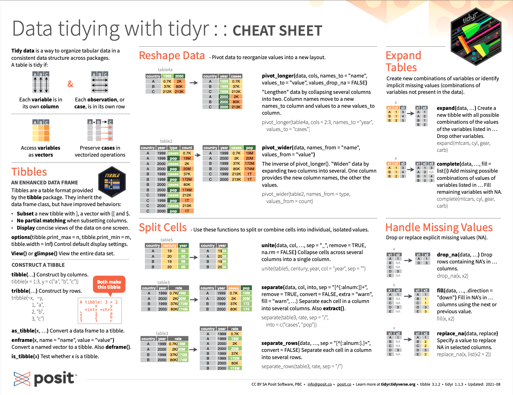
Figure 14.1: The RStudio cheatsheet on tidying data with tidyr functions.

For background information on the notion of tidy data, see the following paper by Hadley Wickham (2014b):
- Wickham, H. (2014). Tidy data. Journal of Statistical Software, 59(10), 1–23. doi: 10.18637/jss.v059.i10 (available at https://www.jstatsoft.org/article/view/v059i10)

For a critical view, see the following blog post:
- What is “tidy data”? (by John Mount)

14.3.3 Preview

Given that we now can read or create data tables, and transform them with both dplyr and tidyr, we now have all ingredients in place for conducting an exploratory data analysis (EDA). Thus, Chapter 15) will be on exploring data.

14.4 Exercises

Some of the following exercises on reshaping tables with tidyr (Wickham & Girlich, 2024) are based on Chapter 7: Tidying data of the ds4psy book (Neth, 2023a):

14.4.1 Four messes and one tidy table

Exercise 1

14.4.2 Moving stocks (from wide to long to wide)

Exercise 2

14.4.3 Reshaping Anscombe’s quartet

Recall Anscombe’s quartet from Chapter 7 on Visualize: Why and how? (see Section 7.2.1). The anscombe data of the datasets package contains the four sets as corresponding $x$- and $y$-variables of an R data frame.

Use tidyr functions to turn this data from its wide format into long format.
Turn your solution from its wide format back into the original long format.
Bonus task: Re-solve 1. by using a different tidyr function.
Bonus task: Re-solve 2. by using a different tidyr function.

Hint: The anscombe data contains 11 rows (observations) and 8 columns (variables). In a long format with two main variables ($x$ and $y$), this would require 44 rows, plus one numeric helper variable denoting the set. Thus, we are aiming for a 44-by-3 data frame.

14.4.4 Comparing numeracy and IQ scores

The tibble exp_num_dt (provided by the ds4psy package) contains data that describe the numeracy (as measured by the Berlin numeracy test, BNT, see http://www.riskliteracy.org/ for details) and IQ scores of 1000 fictitious, but pleasingly open-minded people.

Compute and visualize the average numeracy scores (for all four BNT variables) by participants’ gender.
Compute and visualize the average IQ scores (for general vs. social IQ) by participants’ blood type.
Bonus task: Compute and visualize the relationship between participants’ overall numeracy and their IQ scores.

Do these overviews suggest any systematic patterns in the data?

Hint: Some of these tasks first require selecting the relevant variables and then re-shaping the remaining table from a wide into a longer format. Use pipes of dplyr and tidyr functions for selecting and re-shaping the data and then create appropriate summary tables (e.g., by using dplyr) and visualizations (e.g., bar or boxplots using ggplot2).

Solution

Suitable visualizations to address these tasks could look as follows:

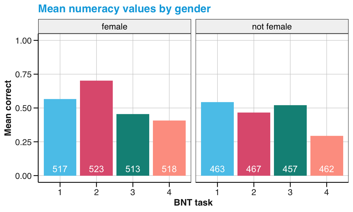
Figure 14.2: Mean numeracy performance by gender. (Labels in white indicate the number of observations.)

Mean IQ values by blood type. (Note that the range of y-axis values has been truncated. Labels in white indicate the number of observations.)

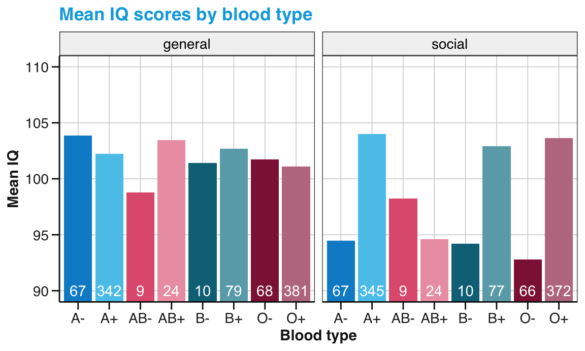
Figure 14.3: Mean IQ values by blood type. (Note that the range of y-axis values has been truncated. Labels in white indicate the number of observations.)

Mean IQ values by mean numeracy score. (Note that the range of y-axis values has been truncated. Labels in white indicate the number of observations.)

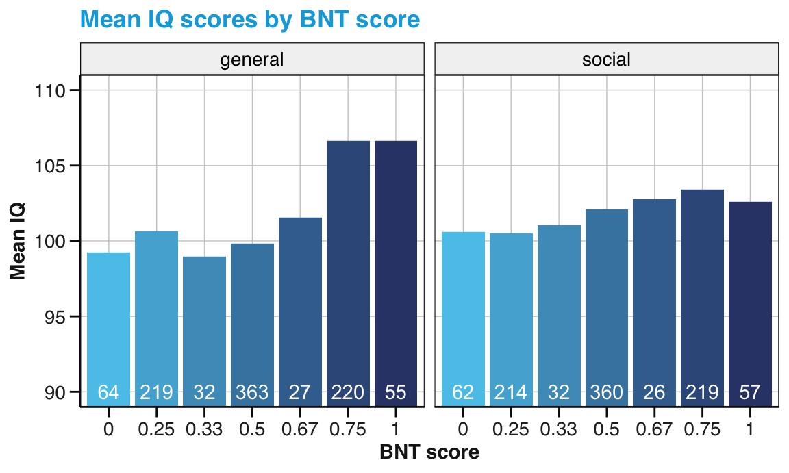
Figure 14.4: Mean IQ values by mean numeracy score. (Note that the range of y-axis values has been truncated. Labels in white indicate the number of observations.)

14.4.5 Plotting relatives

Exercise 5

14.4.6 Widening rental accounting

In Exercise 2 of Chapter 5: Tibbles of the ds4psy book, we recorded the household purchases of the following table:

Name	Mon	Tue	Wed	Thu	Fri	Sat	Sun
Anna	Bread: $2.50	Pasta: $4.50	Pencils: $3.25	Milk: $4.80	–	Cookies: $4.40	Cake: $12.50
	Butter: $2.00						Cream: $3.90
Brian	Chips: $3.80	Beer: $11.80	Steak: $16.20	–	Toilet paper: $4.50	–	Wine: $8.80
Caro	Fruit: $6.30	Batteries: $6.10	–	Newspaper: $2.90	Honey: $3.20	Detergent: $9.95	–

to create a tibble acc_1:

Table 14.5: Table with purchases as observations.
name	day	what	paid
Anna	Mon	Bread	2.50
Anna	Mon	Butter	2.00
Anna	Tue	Pasta	4.50
Anna	Wed	Pencils	3.25
Anna	Thu	Milk	4.80
Anna	Sat	Cookies	4.40
Anna	Sun	Cake	12.50
Anna	Sun	Cream	3.90
Brian	Mon	Chips	3.80
Brian	Tue	Beer	11.80
Brian	Wed	Steak	16.20
Brian	Fri	Toilet paper	4.50
Brian	Sun	Wine	8.80
Caro	Mon	Fruit	6.30
Caro	Tue	Batteries	6.10
Caro	Thu	Newspaper	2.90
Caro	Fri	Honey	3.20
Caro	Sat	Detergent	9.95

In this exercise, we start with the tibble previously created and try to re-create the original table:

In which format is the table acc_1? (Describe acc_1 in terms of its dimensions, variables, and observations.)
Use acc_1 and your knowledge of tidyr to create the (wider) table used in the original exercise (and shown above).

Hint: The resulting tibble (e.g., acc_wider) may contain lists (due to cells containing multiple purchases). However, it is still possible to print such tibbles in R Markdown by using the command knitr::kable(acc_wider).

Solution

This is how a first wider table solution may look like:

Table 14.6: A wider version of the table (with some empty cells and some cells with two elements).
name	Mon	Tue	Wed	Thu	Sat	Sun	Fri
Anna	Bread: $2.5, Butter: $2	Pasta: $4.5	Pencils: $3.25	Milk: $4.8	Cookies: $4.4	Cake: $12.5, Cream: $3.9	NULL
Brian	Chips: $3.8	Beer: $11.8	Steak: $16.2	NULL	NULL	Wine: $8.8	Toilet paper: $4.5
Caro	Fruit: $6.3	Batteries: $6.1	NULL	Newspaper: $2.9	Detergent: $9.95	NULL	Honey: $3.2

A wider table may be easier to read for humans (with a habit of categorizing their social world into people and perceiving time in days of weeks) but is harder to process (e.g., for computers). Note, however, that the order of days within a week does not yet conform to our usual convention. Why is that? And how could it be fixed?

14.4.7 Bonus task: Transposing a data frame

Assume a data frame df and implement a transpose() function that combines gather() and spread() pipes to swap its rows and columns (similar to what the base R function t() does for matrices).

13 Transforming data

15 Exploring data

14 Tidying data

Preparation

Preflections

14.1 Introduction

14.1.1 Reflection: Same or different data?

14.1.2 Key concepts

14.2 Transforming data with tidyr

14.2.1 What is tidy data?

14.2.2 Essential tidyr functions

14.2.3 Unite variables

14.2.4 Separate variables

14.2.5 Practice: Unite and separate in pipes

Solution

Solution

Solution

14.2.6 Making tables longer

Using gather() for making wide tables longer

Using pivot_longer() rather than gather()

More advanced features of pivot_longer()

14.2.7 Practice: Making tables longer

Solution

Solution

14.2.8 Making tables wider

Using spread() for making long tables wider

Using pivot_wider() rather than spread()

More advanced features of pivot_wider()

14.2.9 Practice: Making tables wider

Solution

Solution

14.3 Conclusion

14.3.1 Summary

14.3.2 Resources

14.3.3 Preview

14.4 Exercises

14.4.1 Four messes and one tidy table

14.4.2 Moving stocks (from wide to long to wide)

14.4.3 Reshaping Anscombe’s quartet

14.4.4 Comparing numeracy and IQ scores

Solution

14.4.5 Plotting relatives

14.4.6 Widening rental accounting

Solution

14.4.7 Bonus task: Transposing a data frame

Using `gather()` for making wide tables longer

Using `pivot_longer()` rather than `gather()`

More advanced features of `pivot_longer()`

Using `spread()` for making long tables wider

Using `pivot_wider()` rather than `spread()`

More advanced features of `pivot_wider()`