22 Social situations
This chapter on social situations continues and extends the topics on modeling and simulations (see Chapters 19 to 21). A new aspect is that we introduce multiple agents that interact with both their environment and with each other. Agents can differ in terms of their goals, their capacities and skills, and their knowledge. Moreover, each agent can experience the other agents as part of its environment. This essentially creates a dynamic simulation in which each agent inhabits a different environment, based on its goals, internal representations, and social experience.
Preflections
What changes when a situation becomes a social one?
What are key characteristics of games?
Are social situations more complex than individual situations?
22.1 Introduction
Consider the following situation: An agent needs to fulfill a mission in a maze of sub-terranean tunnels, but several adversaries are out to kill him. Beyond dexterity and an ability for fast movement, the setting requires a talent for spatial navigation and a keen alertness for observing his enemies which are constantly closing in on him. Before they get too close, he needs to interrupt his mission to kill some of his foes.
If this description made you think of James Bond, you are watching too many agent movies. Actually, they describe Pac-Man, an action game for video arcades developed by the Japanese company Namco and released in 1980 (see Wikipedia). While the idea of a yellow pizza-shaped blob chewing pills and chasing ghosts named Blinky, Inky, and Pinky may not be your first association to “action game”, the game has all ingredients for days of fun.43
Motivation: Computer gaming as fun (i.e., the opposite of work) vs. playing as an essential aspect of human nature.
Clarify key terminology:
social := multiple agents.
games vs. strategic games
Complexity of social situations
22.1.1 What are social situations?
A social situation can turn a game against nature (e.g., an agent exploiting some resource) into a social game (e.g., an agent cooperating or competing with other agents). However, social games do not necessarily replace games against nature, but are typically added to them. This may suggest that social games are necessarily more complex than individual games, and that models of social situations need to be more complex than models of individual agents. Before we dispell this common, plausible, but false stereotype, we need to take a closer look at the concept and nature of games.
From complex games (life, pac man, team sports) to simple games (e.g., rock-paper-scissors, tic-tac-toe, ultimatum game).
What’s the essence of games? Perhaps impossible to define (see Wittgenstein) and may take a lifetime to master (see chess, go, but also sports), but often easy to show and play. Some key elements of games are:
- some goal
- some obstacles (e.g., other agents competing for the same goal)
- some rules
A key aspect of games: Setting and following rules. In order to play, we first need to set and agree on rules. This may sound paradoxical, but following rules is not the opposite of freedom, but the precondition for playing a game.
Define games := freedom to follow rules (see Homo ludens, and corresponding considerations by Schiller and Wittgenstein)
Topics and terms studied by game theory: cooperation/defection, payoff matrices, and equilibria
In Section 21.3, we described the introduction of multiple agents as an additional level of complexity. When it is difficult to describe the interactions between an individual agent and its environemnt, it seems intuitively plausible that adding other agents renders situations more complex. This is due to the fact that considering social situations raises important questions regarding the motivations, relations and interactions between agents (e.g., are they cooperative or competitive?), social influence (intentions and potential for communication and persuasion?), social information (observing behavior or rewards of others?), and joint impact on environment (do more agents improve or deplete resources differently?).
More fundamentally, adding complexity also renders it unclear what we mean by “the environment”. For instance, from the myopic perspective of any individual agent, the beliefs, goals, strategies, and behavior of other agents can be described as part of the social environment. Thus, like the term “background”, our concept of the environment is always relative to our model’s primary focus, target, or “foreground”.
Also, we must not confuse potential complexity with actual complexity. Allowing for social situations mostly adds potential for complexity, but does not necessarily require more complex models. And even when added complexity requires messier models (e.g., to accommodate changes on additional dimensions), this does not necessarily render life more challenging for agents. For instance, copying the behavior of others can be much simpler than learning what’s best in an environment. Given some boundary conditions, simple strategies can be both smart (when others are well-adapted) or stupid (when superior solutions exist).
Actually, the potential of simple models for complex phenomena should not surprise us. Note that a theory of Pavlovian learning can be fairly successful by only using terms like “dog”, “bell” and “food” (or technical terms like UCS, CS). Importantly, a model of learning can be very good at both describing and predicting the dog’s behavior without modeling complex interactions in neuronal networks.44
Thus, social games allow for more potential complexity (i.e., interactions of agents with environments and with each other). However, from an agent’s or the modeler’s perspective, this does not necessarily make them more complex.
22.1.2 Models of social situations
The basic models of agents and environments discussed in the previous chapter (see Chapter 21 on Dynamic simulations) were typically developed for individuals. For instance, the framework of reinforcement learning (RL, or the more general class of Markov Decision Processes, MDPs) allows an agent to learn a strategy that maximizes some reward in a stable environment. The options in this environment may be stochastic (e.g., a multi-armed bandit, MAB). Provided that the agent has sufficient time to explore all options, the agent is guaranteed to find the best option. However, if fundamental aspects of the environment change (e.g., by adding options or changing their reward functions), a learning agent may no longer converge on the best option.
Social situations typically change an environment in several ways. Depending on the details of the agent-environment interaction (e.g., how are rewards distributed), they may introduce competition between agents, opportunities for cooperation, and new types of information and learning. For instance, the success of any particular agent strategy can crucially depend on the strategies of other agents. Thus, allowing for other agents questions many results that hold for individual situations and calls for additional types of models and modeling.
In this chapter, we provide a glimpse on some important families of models. Specifically, we introduce three basic paradigms of modeling social situations:
22.2 Games
We first define what the scientific discipline of game theory means by a game.
22.2.1 Terminology
The scientific discipline of game theory has little resemblance to childrens’ games, but instead studies mathematical models of strategic interactions among rational decision-makers (see Wikipedia). In a similar vein, the Stanford Encyclopedia of Philosophy defines game theory as
… the study of the ways in which interacting choices of economic agents
produce outcomes with respect to the preferences (or utilities) of those agents,
where the outcomes in question might have been intended by none of the agents.Ross (2019)
The article immediately adds that the meaning of this definition requires an understanding of the italicized concepts (and provides these details in the corresponding article). For us, it is interesting that games are expressed in terms of economic exchanges, involving agents that pursue their goals, but may obtain outcomes that also depend on the goals and actions of other agents.
We can define a game as a payoff matrix that shows the options and corresponding rewards for its players (in terms of points gained or lost for each combination of outcomes).
One of the simplest possible games is illustrated by Table 22.1. In the matching pennies (MP) game, two players each select one side of a coin (i.e., heads H, or tails T). One player wins if both sides match, the other player wins whenever both sides differ. The payoff matrix shown in Table 22.1 illustrates the options of Player 1 as rows and the first payoff value in each cell, whereas the options of Player 2 are shown as columns and the second payoff values. Thus, Player 1 wins a point (\(+1\)) and Player 2 loses a point (\(-1\)) whenever both players selected the same side of their coins (“HH” or “TT”). Player 2 wins a point (\(+1\)) and Player 1 loses a point (\(-1\)) whenever both players selected different sides of their coins (“HT” or “TH”).
| Options | H | T |
|---|---|---|
| H | \((+1, -1)\) | \((-1, +1)\) |
| T | \((-1, +1)\) | \((+1, -1)\) |
Winning a game can correspond to maximizing one’s individual reward in a game or to gaining more reward than other players of the same game. As the outcome of any single game may be highly dependent on chance factors, the success of a game-playing strategy is typically assessed over repeated instances of the same game. The goal of maximizing one’s own rewards can create dilemmas when contrasting different levels of aggregation (e.g., single vs. repeated games, or individual vs. population gains).
22.2.2 Game types
Different games can be classified into types by comparing the players’ reward functions. The most important types of games are:
zero-sum or pure competitive games: Some player’s wins correspond to another player’s losses, so that the total of all rewards add up to zero (0).
common interest, identical or symmetrical games: All players have the same reward function
general sum games: An umbrella category for other games (i.e., not of the other types).
Note that these categories are not mutually exclusive. For instance, the matching pennies game (shown in Table 22.1) is a symmetrical, purely competitive, zero-sum game. If one player’s win did not correspond to the other player’s loss (e.g., all payoffs of \(-1\) were replaced by payoffs of \(0\)), the game is no longer a zero-sum game, but would still be a symmetrical, common interest game.
To provide a contrast to the competitive matching pennies game, Table 22.2 shows a coordination game. As both players still have identical payoffs, this is a symmetrical common interest game in which both players win by choosing the same side of their coins. Note that there are two different local maxima in this game: As long as both options match, no player is motivated to alter her or his choice. The notion of using the best response given the current choices of other players is an important solution concept in game theory, known as the Nash equilibrium (NE). In the coordination game defined by Table 22.2, the payoffs for TT are higher than for HH, but if a player has reasons to assume that the opponent will choose H, then selecting H is better than insisting on T.
| Options | H | T |
|---|---|---|
| H | \((1, 1)\) | \((0, 0)\) |
| T | \((0, 0)\) | \((2, 2)\) |
See Nowé et al. (2012), for the payoff matrices and descriptions of additional types of games. (We will address the prisoner’s dilemma, PD, and the battle of the sexes, BoS, game in Exercise 22.6.3.)
Games can be further characterized by the order of play (i.e., whether players make sequential vs. simultaneous moves) and by the challenges they pose to their players (e.g., competitive vs. coordination games). Most games assume some balanced and shared understanding of a game’s goals and rules (e.g., all players may either know their own options and payoffs, or even know the full payoff matrix). However, different games and different versions of the same game can differ substantially in the transparency of players’ actions, rewards, and strategies.
A key aspect in modeling games concerns each player’s knowledge of the goals, actions, and rewards of other players. From a modeler’s perspective, we must be aware which aspect of a potentially complex situation is being addressed by a model. This essentially boils down to asking: Which research question is being addressed by modeling this game?
22.2.3 Learning in games
A game can be viewed as a learning environment: A player’s task is to play the game more successfully and increase her chances of winning the game.
Given our experience in modeling dynamic agents and environments (from Chapter 21), we may not need any new tools to model strategic games.
From the perspective of a player (e.g., a RL agent), the strategy and behavior of other players are part of the environment.
To do something more interesting, we will adopt a simulation created by Wataru Toyokawa (which can be found here). This will be a bit challenging, but extend our previous models in three useful ways:
Rather than simulating the repeated encounters of two individuals, we will simulate a spatial population of agents in a lattice/torus design.
Rather than using our basic learning model from Section 21.2, we implement a more sophisticated learning model: An epsilon-greedy Q learning model, which uses a softmax criterion for choosing options.
Given that we are simulating a spatially arranged population of agents over time, we will visualize their choices as an animation.
Methodologically, the extension from individual agents to an entire population of learning agents also motivates some 3-dimensional data structures (i.e., arrays) that provide slots for each agent/player \(p\) and time step \(t\)).
Basic setup
- Defining the game:
# Game:
N_opt <- 2  # Number of options

# Payoff matrix (per player) of the coordination game:
payoff_p1 <- matrix(c(1, 0, 0, 2), nrow = N_opt, byrow = TRUE)  # Player 1
payoff_p2 <- matrix(c(1, 0, 0, 2), nrow = N_opt, byrow = TRUE)  # Player 2

get_payoffs <- function(opt_p1, opt_p2){

  # Look up values in matrices:
  pay_p1 <- payoff_p1[opt_p1, opt_p2]
  pay_p2 <- payoff_p2[opt_p1, opt_p2]

  pay_offs <- c(pay_p1, pay_p2)

  return(pay_offs)
}

## Check:
# get_payoffs(2, 2)- Simulation parameters:
- simulating a population of individuals, arranged in square (a so-called lattice or torus)
Basic idea: Approximating the dynamics of a large (ideally infinite) system by simulating a spatial grid of its parts.
In each round, each individual plays against its 8 neighbors (defined as either sharing a side or a corner with the focal individual).
Boundary condition: Individuals on the edge(s) play against those on the edge of the opposite side (bottom vs. top, left vs. right).
LAT <- 10     # length/width of lattice
N_p <- LAT^2  # population size/number of players
N_t <- 100    # number of games/rounds/time steps

# The boundary condition of the lattice/torus:
boundary_cond <- function(i) { # i is x or y coordinate:

  if (i < 1) {

    return (i + LAT)

  } else if (i > LAT) {

    return (i - LAT)

  } else {

    return (i)

  }
}
Figure 22.1 shows the resulting structure of 100 individuals. In each round, the focal individuals in the darker (blue/green/pink) color play their eight neighbors in lighter (blue/green/pink) color.
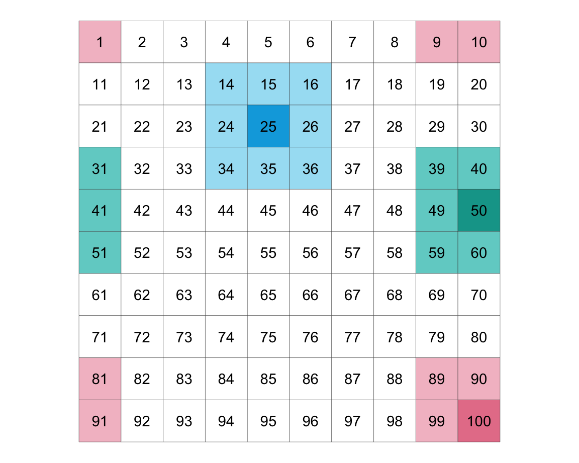
Figure 22.1: Illustrating a torus structure of 100 individuals arranged on a 10x10 lattice.
Consequences
The lattice/torus design creates a spatial continuum of agents, and strategies, and interactions. From the perspective of each individual agent, this setup multiplies the number of games she plays and the diversity of strategies she encounters. From the modeler’s perspective, this setup allows assessing the density of each strategy at each point in time, as well as the diffusion of strategies over time. Under some circumstances, a global pattern may emerge out of local interactions.
- Some utility functions:
# exp_ceiling() limits the exponential of x
# to a maximum value of 2^1023:
exp_ceiling <- function(x) {

  exp_x <- exp(x)  # compute exp once

  ix_inf <- which(is.infinite(exp_x))  # ix of infinite values

  if (length(ix_inf) == 0) {

    return(exp_x)  # return as is

  } else { # limit infinite values:

    exp_x[ix_inf] <- 8.988466e+307  # 2^1023

    return(exp_x)

  }
}

## Check:
# x <- c(10, 100, 1000)  # Note: exp(710) => Inf
# exp(x)
# exp_ceiling(x)

# Simple vector calculation functions (to use in apply()):
divide_vec = function (num, den) {

  return(num/den)

}

multiply_vec = function (Q, beta) {

  return(Q * beta)

}- Set learner parameters:
# Learner:
epsilon   <- 0.1  # exploration rate (epsilon-greedy model)
alpha     <- 0.5  # learning rate/step size parameter
Q_initial <- 0    # initial payoff expectation
Q         <- array(dim = c(N_opt, N_t, N_p))
Q[ , 1, ] <- Q_initial
Note the 3-dimensional array of Q values (with dimensions of N_opt, N_t, and N_p, i.e., providing 2 x 100 x 100 slots).
- Prepare data structures for storing intermediate results:
# Storing history:
choices       <- matrix(nrow = N_p, ncol = N_t)  # in wide format
payoffs       <- matrix(nrow = N_p, ncol = N_t)
performance   <- matrix(nrow = N_p, ncol = N_t)

choiceCounter   <- array(0, dim = c(N_opt, N_p))
riskyChoiceProb <- matrix(nrow = N_p, ncol = N_t)
netChoiceProb   <- array(dim = c(N_opt,  N_t, N_p))
netChoiceProb[ , 1, ] <- 1/N_opt

density_1 <- rep(NA, N_t)
density_2 <- rep(NA, N_t)

# this is a list where the tactics distribution of each time step will be recorded
all_choices <- list()
Simulation
Running the simulation as a for loop (for each time step \(t\)):
for (t in 1:N_t) {

  # Each individual chooses one option based on his/her choice probability netChoiceProb[ , t, ]:
  choices[ , t] = apply(netChoiceProb[ , t, ], MARGIN = 2,
                        FUN = function(netChoiceProbInstance){
                          sample(1:N_opt, 1, prob = netChoiceProbInstance, replace = FALSE)})

  all_choices$step[[t]] <- matrix(choices[ , t], nrow = LAT, ncol = LAT, byrow = TRUE)

  # Calculate the density of each option:
  density_1[t] <- which(choices[ , t] == 1) %>% length() %>% divide_vec(., LAT^2)
  density_2[t] <- which(choices[ , t] == 2) %>% length() %>% divide_vec(., LAT^2)
  # OR: # density_2[t] <- 1 - density_1[t]

  # Calculate payoffs of each player:
  # Assumption: Each player plays the game once against each of the 8 neighbors:
  for (p in 1:N_p) {

    # the position (address?) of the focal player in the lattice:
    i <- (p - 1) %/% LAT + 1  # quotient
    j <- (p - 1) %%  LAT + 1  # remainder
    payoffs[p, t] <- 0        # initialize value

    for (g in c(-1, 0, 1)) {  # neighbor x
      for (h in c(-1, 0, 1)) {  # neighbor y

        if (g^2 + h^2 > 0) {  # is FALSE iff g == h == 0, which eliminates the focal player:

          # Determine current payoffs (given player choices):
          cur_payoffs <- get_payoffs(opt_p1 = all_choices$step[[t]][i, j],
                                     opt_p2 = all_choices$step[[t]][boundary_cond(i+g), boundary_cond(j+h)])

          cur_payoff_p1 <- cur_payoffs[1]  # payoff of focal player

          payoffs[p, t] <- payoffs[p, t] + cur_payoff_p1  # accumulate payoffs of focal player

        } # if.

      } # for h.
    } # for g.

  } # for p.

  # cur_choices tracks which option was chosen by each individual on this trial:
  cur_choices <- choices[ , t] + N_opt * (1:N_p - 1)

  # Updating Q values (only if another trial is following):
  if (t < N_t) {

    # Copying the previous Q value to the current Q value:
    Q[ , t + 1, ] <- Q[ , t, ]

    QQ <- aperm(Q, c(1, 3, 2))  # transpose dimensions 2 and 3 of Q
    dim(QQ) <- c(N_opt * N_p, N_t)

    # Q value updating (note: alpha is a step-size parameter which is 1/n; the sample averaging rule):
    QQ[cur_choices, t + 1] <- QQ[cur_choices, t] + alpha * (payoffs[ , t] - QQ[cur_choices, t])

    dim(QQ) <- c(N_opt, N_p, N_t)
    Q <- aperm(QQ, c(1, 3, 2))


    # Softmax choice (based only on Q values): ----

    Q_exp <- (Q[ , t + 1, ] * rep(20, each = N_opt)) %>%
      apply(., MARGIN = 2, FUN = exp_ceiling) %>% round(., 5)

    softmaxMatrix <- Q_exp %>%
      apply(1, divide_vec, den = apply(Q_exp, MARGIN = 2, FUN = sum)) %>%
      t() %>% round(., 5)

    # Softmax end.


    # Update choice probability matrix: ----
    netMatrix <- apply(X = softmaxMatrix, MARGIN = 1, FUN = multiply_vec, beta = (1 - epsilon)) %>%
      t() + apply(matrix(rep(1/N_opt, N_opt * N_p), N_opt:N_p), MARGIN = 1, FUN = multiply_vec, beta = epsilon) %>%
      t() %>% round(., 4)

    netChoiceProbAperm      <- aperm(netChoiceProb, c(1, 3, 2))
    dim(netChoiceProbAperm) <- c(N_opt * N_p, N_t)
    dim(netMatrix)          <- c(N_opt * N_p, 1)
    netChoiceProbAperm[ , t + 1] <- netMatrix
    dim(netChoiceProbAperm)      <- c(N_opt, N_p, N_t)
    netChoiceProb                <- aperm(netChoiceProbAperm, c(1, 3, 2))

  } # if (t < N_t).

} # for t.
Note some assumptions:
- Each player selects her choice once at the beginning of each trial. Thus, it does not consider its opponents individually.
Results
Visualizing results for a population of agents requires calculating the density of their choices, rather than individual ones.
This is why we computed the density_1 and density_1 vectors during the simulation:
- Density dynamics of option choices over 100 trials:
# Prepare data frame:
density_data <- data.frame(t = 1:N_t,
                           density_1 = density_1,
                           density_2 = density_2)

density_long <- density_data %>%
  pivot_longer(cols = c(-t), names_to = 'option', values_to = 'density')

ggplot(density_long) +
  geom_hline(yintercept = 1/N_opt, linetype = 'dashed', color = "grey50")+
  geom_line(aes(t, density, color = option), size = 1, alpha = 3/4)+
  scale_color_manual(values = c('density_1' = usecol(Pinky),
                                'density_2' = usecol(Seeblau)),
                     labels = c("Option 1", "Option 2")) +
  ylim(c(0, 1)) +
  labs(title = "Density dynamics of options over time",
       x = "Time step t", y = "Option density", color = "Options:") +
  theme_ds4psy()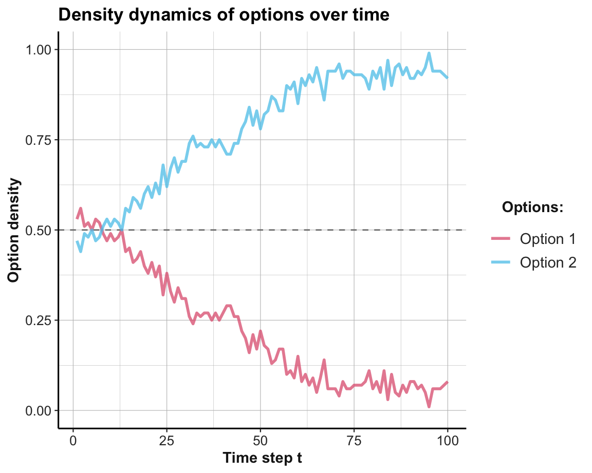
Creating an animated plot
To visualize the spatical dynamics of agent choices over time, we can show which opten each agent on the lattice/torus has chosen on every trial. This can be visualized as an animated gif, in two steps:
- Prepare data: Transform the 3-dimensional array of
all_choicesinto a 2-dimensional tableall_choices_tb
for (t in 1:N_t) {

  matrix <- as_tibble(all_choices$step[[t]], .name_repair = "unique")
  names(matrix) <- as.character(1:LAT)
  matrix$y <- 1:LAT

  if (t == 1) {

    all_choices_tb <- matrix %>%
      pivot_longer(cols = c(-y), names_to = 'x', values_to = 'option')
    all_choices_tb$x <- as.numeric(all_choices_tb$x)
    all_choices_tb$trial <- rep(t, LAT^2)

  } else {

    all_choices_tb_temp <- matrix %>%
      pivot_longer(cols = c(-y), names_to = 'x', values_to = 'option')
    all_choices_tb_temp$x <- as.numeric(all_choices_tb_temp$x)
    all_choices_tb_temp$trial <- rep(t, LAT^2)

    all_choices_tb <- rbind(all_choices_tb, all_choices_tb_temp)

  } # if.
}

# Check result:
dim(all_choices_tb)
#> [1] 10000     4
head(all_choices_tb)
#> # A tibble: 6 × 4
#>       y     x option trial
#>   <int> <dbl>  <int> <int>
#> 1     1     1      2     1
#> 2     1     2      2     1
#> 3     1     3      1     1
#> 4     1     4      1     1
#> 5     1     5      2     1
#> 6 1 6 2 1- Create an animated image (by using the gganimate and gifski packages):
library(gganimate)
library(gifski)

animate_choices <- all_choices_tb %>%
    ggplot() +
    geom_raster(aes(x, y, fill = as.factor(option)))+
    scale_fill_manual(values = c('1' = pal_pinky[[3]], '2' = pal_seeblau[[3]]),
                      labels = c("Option 1", "Option 2")) +
    scale_x_continuous(breaks = 1:10, labels = 1:10) +
    scale_y_continuous(breaks = 1:10, labels = 1:10) +
    coord_equal() +
    theme_ds4psy() +
    # gganimate-specific parts:
    transition_time(trial) +
    labs(title = "Trial {frame_time} of a coordination game",
         fill = "Options:", x = "", y = "") +
    ease_aes("linear")

animate(animate_choices, duration = 10, fps = 10,
        width = 400, height = 400, renderer = gifski_renderer())

# anim_save("images/soc_anim_coord.gif")  # save image
The resulting Figure 22.2 shows that both options are equally prominent at first, but the superior Option 2 is becoming more popular from Trial 10 onwards. Due to the agents’ tendency to explore, Option 1 is still occasionally chosen.

Figure 22.2: The distribution of agent choices over time in the coordination game.
Practice
This exercise adjusts the simulation of the coordination game to the matching pennies (MP) game (defined by Table 22.1):
What is the optimal strategy that agents should learn in a purely competitive game?
What needs to be changed to use the above model to simulate this game?
Adopt the simulation to verify your answers to 1. and 2.
Solution
ad 1.: As any predictable agent could be exploited, the optimal choice for an individual agent is to randomly choose options. However, it is unclear what this would mean for a population of agents arranged on a lattice/torus.
ad 2.: Theoretically, we only need to re-define the payoff matrix of the game (shown in Table 22.1). However, as the model above yields an error (when converting negative payoffs into probabilities), we add 1 to all payoffs. This turns a zero-sum game into a competitive game with symmetrical payoffs, but has no effect on the absolute differences in payoffs that matter for our RL agents):
# Payoff matrix (per player) of a competitive (matching pennies, MP) game:
payoff_p1 <- matrix(c(1, -1, -1, 1), nrow = N_opt, byrow = TRUE) + 1  # Player 1
payoff_p2 <- matrix(c(-1, 1, 1, -1), nrow = N_opt, byrow = TRUE) + 1 # Player 2- ad 3.: Figure 22.3 shows the result of a corresponding simulation. In this particular simulation, a slight majority of agents chose Option 1, but the population did not reach a stable equilibrium. As each agent’s optimal strategy is to choose options randomly (i.e., with a \(p=.5\) for each option), this could be evidence for learning. But to really demonstrate successful learning, further examinations would be necessary.
Figure 22.3: The distribution of agent choices over time in a competitive game.
22.3 Social learning
Learning can be modeled as a function of rewards and the behavior of others. When an option is better than another, it offers higher rewards and will be learned by an agent that explores and exploits an environment to maximize her utility. However, when other agents are present, a second indicator of an option’s quality is its popularity: Other things being equal, better options are more popular.45
22.3.1 Replicator dynamics
The basic idea of replicator dynamics (following Page, 2018, p. 308ff.) is simple: The probability of choosing an action is the product of its reward and its popularity.
Given a set of \(N_opt\) alternatives with corresponding rewards \(\pi(1) ... \pi(n)\), the probability of choosing an option \(k\) at time step \(t+1\) is defined as:
\[ P_{t+1}(k) = P_{t}(k) \cdot \frac{\pi(k)}{\bar{\pi_{t}}}\]
Note that the factor given by the fraction \(\frac{\pi(k)}{\bar{\pi_{t}}}\) divides the option’s current reward by the current average reward of all options. Its denominator is computed as the sum of all reward values weighted by their probability in the current population. As more popular options are weighted more heavily, this factor combines an effect of reward with an effect of popularity or conformity. Thus, the probability of choosing an option on the next decision cycle depends on its current probability, its current reward, and its current popularity.
Note that this particular conceptualization provides a model for an entire population, rather than any individual element of it. Additionally, the rewards received from each option are assumed to be fixed and independent of the choices, which may be pretty implausible for many real environments.
What changes would signal that the population is learning? The probability distribution of actions being chosen in each time step.
Implementation in R
# Environment parameters:
alt  <- c("A", "B", "C")
rew  <- c(20, 10, 5)
prob <- c(.1, .7, .2)  # initial probability distribution
N_t  <- 10  # number of time steps/rounds/trials

# Prepare data storage:
data <- as.data.frame(matrix(NA, ncol = 5, nrow = 10 + 1))
names(data) <- c("t", "avg_rew", paste0("p_", alt))

for (t in 0:N_t){

  # (1) Compute average reward:
  avg_rew <- sum(prob * rew)

  # (+) User feedback/data storage:
  # print(paste0(t, ": avg_rew = ", round(avg_rew, 1),
  #              ": prob = ", paste0(round(prob, 2), collapse = ":")))
  data[(t + 1), ] <- c(t, round(avg_rew, 2), round(prob, 3))

  # (2) Update probability:
  prob <- prob * rew/avg_rew

}
Given that we collected all intermediate values in data, we can inspect our simulation results by printing the table:
| t | avg_rew | p_A | p_B | p_C |
|---|---|---|---|---|
| 0 | 10.00 | 0.100 | 0.700 | 0.200 |
| 1 | 11.50 | 0.200 | 0.700 | 0.100 |
| 2 | 13.26 | 0.348 | 0.609 | 0.043 |
| 3 | 15.16 | 0.525 | 0.459 | 0.016 |
| 4 | 16.89 | 0.692 | 0.303 | 0.005 |
| 5 | 18.18 | 0.819 | 0.179 | 0.002 |
| 6 | 19.01 | 0.901 | 0.099 | 0.000 |
| 7 | 19.48 | 0.948 | 0.052 | 0.000 |
| 8 | 19.73 | 0.973 | 0.027 | 0.000 |
| 9 | 19.87 | 0.987 | 0.013 | 0.000 |
| 10 | 19.93 | 0.993 | 0.007 | 0.000 |
As shown in Table 22.3, we initialized our loop at a value of t = 0.
This allowed us to include the original situation (prior to any updating of prob) as the first line
(i.e., in row data[(t + 1), ]).
Inspecting the rows of Table 22.3 makes it clear that the probabilities of suboptimal options (here: Options B and C) are decreasing, while the probability of choosing the best option (A) is increasing. Thus, options with higher rewards are becoming more popular — and the population quickly converges on choosing the best option.
The population’s systematic shift from poorer to richer options also implies that the value of the average reward (here: avg_rew) is monotonically increasing and approaching the value of the best option. Thus, the function of avg_rew is similar to the role of an aspiration level \(A\) in reinforcement learning models (see Section 21.2), with the difference that avg_rew reflects the average aspiration of the entire population, whereas \(A_{i}\) denotes the aspiration level of an individual agent \(i\).
Visualizing results
Ways of depicting the shift in collective dynamics away from bad and towards the best option is provided by the following visualizations of data.
Figure 22.4 shows the trends in choosing each option as a function fo the time steps 0 to 10:
library(tidyverse)
library(ds4psy)
library(unikn)

# Re-format data:
data_long <- data %>%
  pivot_longer(cols = starts_with("p_"),
               names_to = "option",
               values_to = "p") %>%
  mutate(opt = substr(option, 3, 3))
# data_long

ggplot(data_long, aes(x = t, y = p, group = opt, col = opt)) +
  geom_line(size = 1.5, alpha = .5) +
  geom_point(aes(shape = opt), size = 2) +
  scale_y_continuous(labels = scales::percent_format()) +
  scale_x_continuous(breaks = 0:10, labels = 0:10) +
  scale_color_manual(values = usecol(c(Seegruen, Seeblau, Pinky))) +
  labs(title = paste0("Probability trends over ", N_t, " steps"),
       x = "Time steps", y = "Probability",
       col = "Option:", shape = "Option:") +
  theme_ds4psy()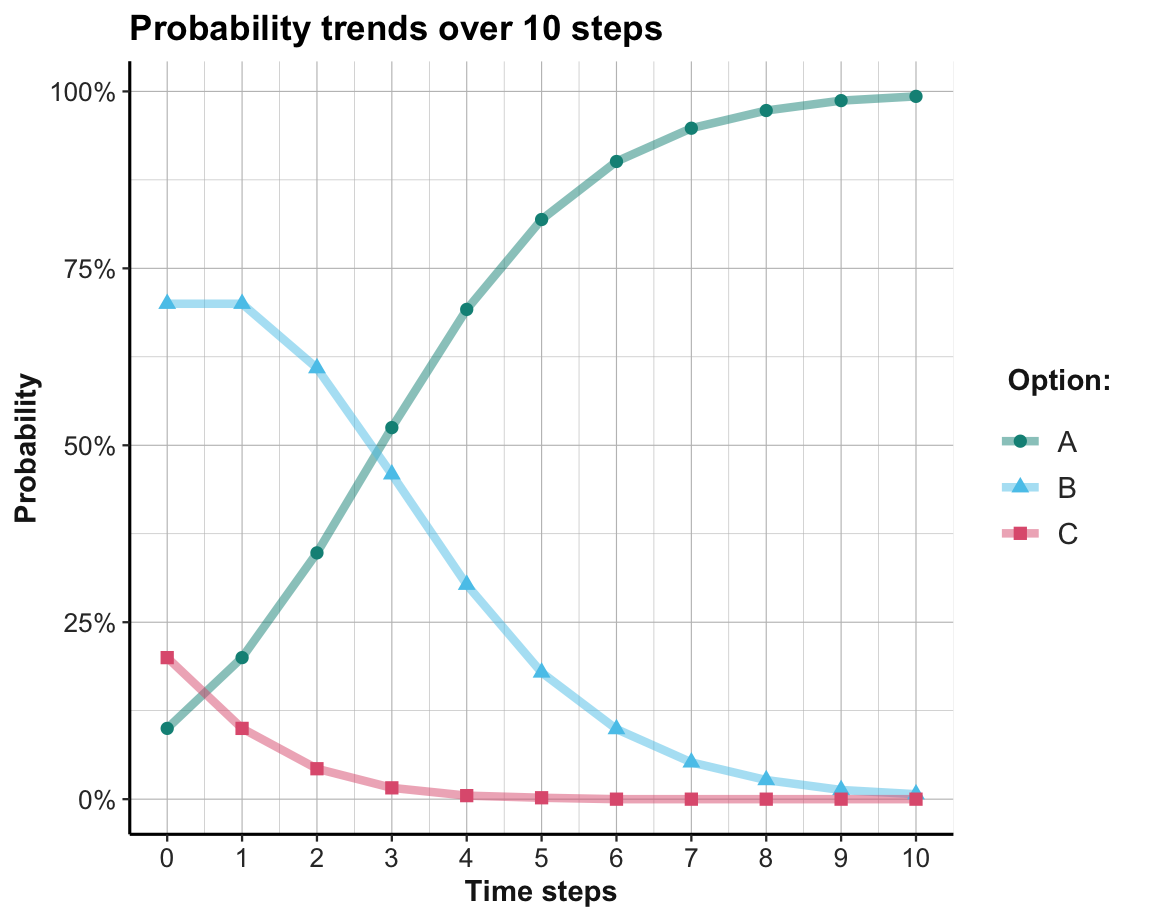
Figure 22.4: Trends in the probabilty of choosing each option per time step.
Note that we re-formatted data into long format prior to plotting (to get the options as one variable, rather than as three separate variables) and changed the y-axis to a percentage scale.
Given that the probability distribution at each time step must sum to 1, it makes sense to display them as a stacked bar chart, with different colors for each option (see Figure 22.5):
ggplot(data_long, aes(x = t, y = p, fill = opt)) +
  geom_bar(position = "fill", stat = "identity") +
  scale_y_continuous(labels = scales::percent_format()) +
  scale_x_continuous(breaks = 0:10, labels = 0:10) +
  scale_fill_manual(values = usecol(c(Seegruen, Seeblau, Pinky))) +
  labs(title = paste0("Probability distributions over ", N_t, " steps"),
       x = "Time steps", y = "Probability",
       col = "Option:", fill = "Option:") +
  theme_ds4psy()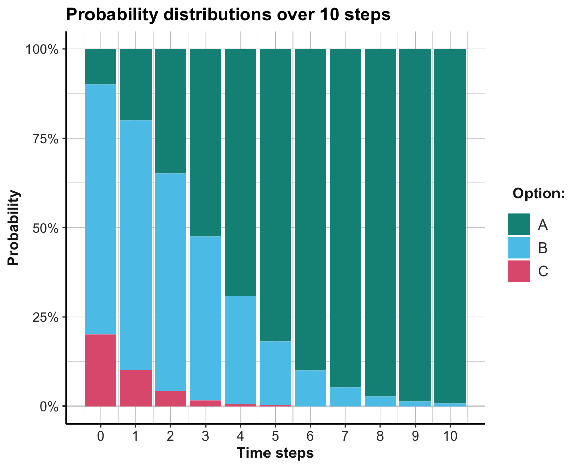
Figure 22.5: The probabilty of choosing options per time step.
This shows that the best option (here: Option A) is unpopular at first, but becomes the dominant one by about the 4-th time step. The learning process shown here appears to be much quicker than that of an individual reinforcement learner (in Section 21.2). This is mostly due to a change in our level of analysis: Our model of replicator dynamics describes an entire population of agents. In fact, our use of the probability distribution as a proxy for the popularity of options implicitly assumes that an infinite population of agents is experiencing the environment and both exploring and exploiting the full set of all options on every time step. Whereas an individual RL agent must first explore options and — if it gets unlucky — waste a lot of valuable time on inferior options, a population of agents can evaluate the entire option range and rapidly converge on the best option.
Convergence on the best option is guaranteed as long all options are chosen (i.e., have an initial probability of \(p_{t=0}(i)>0\)) and the population of agents is large (ideally infinite).
Practice
-
Answer the following questions by studying the basic equation of replicator dynamics:
What’s the impact of options that offer zero rewards (i.e, \(\pi(k)=0\))?
What’s the impact of options that are not chosen (i.e, \(P_{t}(k)=0\))?
What happens if the three options (A–C) yield identical rewards (e.g., 10 units for each option)?
-
What happens if the rewards of three options (A–C) yield rewards of 10, 20, and 70 units, but their initial popularities are reversed (i.e., 70%, 20%, 10%).
Do 10 time steps still suffice to learn the best option?
What if the initial contrast is even more extreme, with rewards of 1, 2, and 97 units, and initial probabilities of 97%, 2%, and 1%, respectively?
Hint: Run these simulations in your mind first, then check your predictions with the code above.
-
What real-world environment could qualify as
one in which the rewards of all objects are stable and independent of the agents’ actions?
one in which all agents also have identical preferences?
-
How would the learning process change
if the number of agents was discrete (e.g., 10)?
if the number of options exceeded the number of agents?
Hint: Consider the range of values that prob would and could take in both cases.
22.5 Conclusion
There are many directions for possible extensions:
more complex games (e.g., more agents, options, and outcomes)
more diverse and complex range of interactions
allowing for uncertainty (e.g., in range of options, their likelihoods, and payoff matrices)
22.5.1 Summary
Social situations are often messier than non-social ones, but the corresponding models must not be more complex. In this chapter, the analysis of strategic games, population dynamics, and social networks illustrated some starting points for such models. More detailed models will primarily require a clear conceptual grasp on the research questions to be addressed by them.
22.5.2 Resources

Each main topic of this chapter can easily fill entire books or careers. Here are some pointers to sources of inspirations and ideas:
Games
Axelrod & Hamilton (1981) is a classic on cooperation and the assessment of strategies in a tournament.
Nowé et al. (2012) provide an introduction to game theory and illustrate how reinforcement learning (RL) can be applied to repeated games and Markov games.
Szita (2012) further explores the connections between RL and games.
22.6 Exercises

Ideas for corresponding exercises and projects:
22.6.1 Reflecting on Pac-Man
The video game of Pac-Man is far too fast, rich, and complicated to be modeled as one of our exercises. However, it is instructive to reflect on what would be required to implement a corresponding model.
How could the environment (i.e., the maze, pellets, time steps and rounds) be represented in a computer simulation?
What would a model of the Pac-Man agent require (in terms of goals, internal states, and actions)?
What would change if we were to model the ghosts instead?
Bonus trivia: What is the name of the 4. ghost in Pac-Man?
22.6.2 Bystander intervention and diffusion of responsibility
A famous study on the intervention behavior of bystanders (Darley & Latané, 1968) is often cited as evidence for the so-called “diffusion of responsibility” in helping situations. In fact, the study has shown that individuals are slower to respond to a (fake) emergency situation when they believe to be part of a larger group. However, this finding does not necessarily imply that larger groups are slower to respond than smaller groups or individuals. If it suffices when one member of a group intervenes, a group with some variability in the helping behavior of its members is faster than its average member.
How quickly a group reacts to an emergency depends on parameters of the group (e.g., its size and the similarity of its members) and assumptions about the behavior of its members (e.g., how likely each member is to help, based on parameters of the group). If the helping behavior is modeled probabilistically (e.g., each group member helps with some probability per unit of time), a group could help more quickly even when its average member is helping more slowly.
Conduct simulations to illustrate the helping speed of groups as a function of the behavior of its individual members. Under which conditions are groups faster or slower to help than its average member?
Assuming identical individuals (with a constant probability of helping per unit of time), how does the group helping speed vary as a function of each individual’s helping probability and group size?
Does this result change when each individual’s probability of helping is no longer constant, but drawn from a normal distribution?
22.6.3 Learning in coordination and conflict games
The prisoner’s dilemma (PD) is a notorious example of a two-player coordination game that shows why two rational players may not cooperate, even if it is in their best interests to do so (see Wikipedia for details). Table 22.4 shows a payoff matrix of a PD game.
| Options | cooperate | defect |
|---|---|---|
| cooperate | \((-1, -1)\) | \((-3, +0)\) |
| defect | \((+0, -3)\) | \((-2, -2)\) |
Your tasks:
Classify the PD’s type of game by describing its payoff matrix.
Implement a population of 10 x 10 agents that play the game for 100 rounds (using the lattice/torus setup from Section 22.2). What do they learn? Why?
- Repeat 1. and 2. for the battle of the sexes (BoS) game — a two-player coordination game that pits diverging preferences against each other and thus may involve some conflict (see Wikipedia for details). As the standard version assigns somewhat sexist roles to males and females, Table 22.5 shows a payoff matrix of a BoS game as a dilemma to attend a performance playing either music composed by “Bach” or by “Stravinsky”:
| Options | Bach | Stravinsky |
|---|---|---|
| Bach | \((3, 2)\) | \((0, 0)\) |
| Stravinsky | \((0, 0)\) | \((2, 3)\) |
22.6.4 Playing rock-paper-scissors (RPS)
Table 22.6 illustrates the payoff matrix of the rock-paper-scissors (RPS) game.
| Options | rock | paper | scissors |
|---|---|---|---|
| rock | \((0, 0)\) | \((-1, +1)\) | \((+1, -1)\) |
| paper | \((+1, -1)\) | \((0, 0)\) | \((-1, +1)\) |
| scissors | \((-1, +1)\) | \((+1, -1)\) | \((0, 0)\) |
Classify this type of game and justify your choices by describing the payoff matrix.
What is the most rational strategy when playing this game against an opponent? Why?
Implement the game for a population of 100 agents arranged in a 10 x 10 lattice/torus design, in which each agent plays its 8 surrounding agents on each of \(N_t = 100\) rounds (as in Section 22.2). What do the agents learn?
Hint: This exercise is based on a simulation by Wataru Toyokawa, which can be found here. The original example uses a population of \(42^2 = 1764\) agents, which takes longer, but yields more stable results.
Bonus: Let’s try to reproduce an interesting result based on a Japanese children’s game that uses a biased payoff matrix (see Wataru’s remarks on “Gu-ri-co”).
Assume a RPS game in which each winning player receives the number of points that corresponds to the number of characters in the name of her or his chosen option. This results in a biased payoff matrix that yields 8 points for winning with scissors (asnchar(scissors)is 8), 5 points for winning with paper, and 4 points for winning with rock (and ties and losses earning 1 and 0 points, respectively).Bonus: Assume that your opponent(s) selects her options randomly, but with biased preferences. Specifically, she plays rock on 50% of all trials, paper on 30% of all trials, and scissors on 20% of all trials. Show that and how your learning agent would beat this agent.
Solution
ad 1.: The RPS game is a purely competitive zero-sum game. Its three options are symmetrical in the sense as each option is winning against one and losing against one other option.
ad 2.: The most rational strategy in playing the RPS game is to be maximally unpredictable. This is achieved by selecting each of the three options with a random probability of \(p=1/3\).
ad 3.: We need to re-define the parameters of the game (i.e., options and payoffs), as well as change the auxiliary simulation code to accommodate three options (e.g., their densities).
Here is the resulting code:
Game definition: Change payoff matrices to accommodate three options (and avoid negative payoffs):
# Game:
N_opt <- 3  # NEW: Number of options

# NEW payoff matrices (per player) of the RPS game:
payoff_p1 <- matrix(c( 0, -1, +1,
                      +1,  0, -1,
                      -1, +1,  0),
                    nrow = N_opt, byrow = TRUE)  # Player 1 payoffs
payoff_p2 <- -1 * payoff_p1  # Player 2 payoffs

# HACK to avoid negative payoffs (NEW):
payoff_p1 <- payoff_p1 + 1
payoff_p2 <- payoff_p2 + 1

get_payoffs <- function(opt_p1, opt_p2){

  # Look up values in matrices:
  pay_p1 <- payoff_p1[opt_p1, opt_p2]
  pay_p2 <- payoff_p2[opt_p1, opt_p2]

  pay_offs <- c(pay_p1, pay_p2)

  return(pay_offs)
}

## Check:
# get_payoffs(3, 1)
Simulation parameters (unchanged):
LAT <- 10     # length/width of lattice
N_p <- LAT^2  # population size/number of players
N_t <- 100    # number of games/rounds/time steps

# The boundary condition of the lattice/torus:
boundary_cond <- function(i) { # i is x or y coordinate:

  if (i < 1) {

    return (i + LAT)

  } else if (i > LAT) {

    return (i - LAT)

  } else {

    return (i)

  }
}
Utility functions (unchanged):
# exp_ceiling() limits the exponential of x
# to a maximum value of 2^1023:
exp_ceiling <- function(x) {

  exp_x <- exp(x)  # compute exp once

  ix_inf <- which(is.infinite(exp_x))  # ix of infinite values

  if (length(ix_inf) == 0) {

    return(exp_x)  # return as is

  } else { # limit infinite values:

    exp_x[ix_inf] <- 8.988466e+307  # 2^1023

    return(exp_x)

  }
}

## Check:
# x <- c(10, 100, 1000)  # Note: exp(710) => Inf
# exp(x)
# exp_ceiling(x)

# Simple vector calculation functions (to use in apply()):
divide_vec = function (num, den) {

  return(num/den)

}

multiply_vec = function (Q, beta) {

  return(Q * beta)

}
Learner parameters (unchanged):
# Learner:
epsilon   <- 0.10  # exploration rate (epsilon-greedy model)
alpha     <- 0.50  # learning rate/step size parameter
Q_initial <- 0     # initial payoff expectation
Q         <- array(dim = c(N_opt, N_t, N_p))
Q[ , 1, ] <- Q_initial
Data structures for storing intermediate results: Adding a density_3 vector to store the probability density of a 3rd option.
# Storing history:
choices       <- matrix(nrow = N_p, ncol = N_t)  # in wide format
payoffs       <- matrix(nrow = N_p, ncol = N_t)
performance   <- matrix(nrow = N_p, ncol = N_t)

choiceCounter   <- array(0, dim = c(N_opt, N_p))
riskyChoiceProb <- matrix(nrow = N_p, ncol = N_t)
netChoiceProb   <- array(dim = c(N_opt,  N_t, N_p))
netChoiceProb[ , 1, ] <- 1/N_opt

density_1 <- rep(NA, N_t)
density_2 <- rep(NA, N_t)
density_3 <- rep(NA, N_t)  # NEW

# this is a list where the tactics distribution of each time step will be recorded
all_choices <- list()
Running the simulation as a for loop (for each time step \(t\)): Adding a line to collect density_3 values on each time step.
for (t in 1:N_t) {

  # Each individual chooses one option based on his/her choice probability netChoiceProb[ , t, ]:
  choices[ , t] = apply(netChoiceProb[ , t, ], MARGIN = 2,
                        FUN = function(netChoiceProbInstance){
                          sample(1:N_opt, 1, prob = netChoiceProbInstance, replace = FALSE)})

  all_choices$step[[t]] <- matrix(choices[ , t], nrow = LAT, ncol = LAT, byrow = TRUE)

  # Calculate the density of each option:
  density_1[t] <- which(choices[ , t] == 1) %>% length() %>% divide_vec(., LAT^2)
  density_2[t] <- which(choices[ , t] == 2) %>% length() %>% divide_vec(., LAT^2)
  density_3[t] <- which(choices[ , t] == 3) %>% length() %>% divide_vec(., LAT^2)  # NEW
  # OR: # density_3[t] <- 1 - (density_1[t] + density_2[t])

  # Calculate payoffs of each player:
  # Assumption: Each player plays the game once against each of the 8 neighbors:
  for (p in 1:N_p) {

    # the position (address?) of the focal player in the lattice:
    i <- (p - 1) %/% LAT + 1  # quotient
    j <- (p - 1) %%  LAT + 1  # remainder
    payoffs[p, t] <- 0        # initialize value

    for (g in c(-1, 0, 1)) {  # neighbor x
      for (h in c(-1, 0, 1)) {  # neighbor y

        if (g^2 + h^2 > 0) {  # is FALSE iff g == h == 0, which eliminates the focal player:

          # Determine current payoffs (given player choices):
          cur_payoffs <- get_payoffs(opt_p1 = all_choices$step[[t]][i, j],
                                     opt_p2 = all_choices$step[[t]][boundary_cond(i+g), boundary_cond(j+h)])

          cur_payoff_p1 <- cur_payoffs[1]  # payoff of focal player

          payoffs[p, t] <- payoffs[p, t] + cur_payoff_p1  # accumulate payoffs of focal player

        } # if.

      } # for h.
    } # for g.

  } # for p.

  # cur_choices tracks which option was chosen by each individual on this trial:
  cur_choices <- choices[ , t] + N_opt * (1:N_p - 1)

  # Updating Q values (only if another trial is following):
  if (t < N_t) {

    # Copying the previous Q value to the current Q value:
    Q[ , t + 1, ] <- Q[ , t, ]

    QQ <- aperm(Q, c(1, 3, 2))  # transpose dimensions 2 and 3 of Q
    dim(QQ) <- c(N_opt * N_p, N_t)

    # Q value updating (note: alpha is a step-size parameter which is 1/n; the sample averaging rule):
    QQ[cur_choices, t + 1] <- QQ[cur_choices, t] + alpha * (payoffs[ , t] - QQ[cur_choices, t])

    dim(QQ) <- c(N_opt, N_p, N_t)
    Q <- aperm(QQ, c(1, 3, 2))

    ###############
    ## Softmax choice (based only on Q values):
    ###############

    Q_exp <- (Q[ , t + 1, ] * rep(20, each = N_opt)) %>%
      apply(., MARGIN = 2, FUN = exp_ceiling) %>% round(., 5)

    softmaxMatrix <- Q_exp %>%
      apply(1, divide_vec, den = apply(Q_exp, MARGIN = 2, FUN = sum)) %>%
      t() %>% round(., 5)

    ###############
    ## Softmax end.
    ###############

    ## Update choice probability matrix:
    netMatrix <- apply(X = softmaxMatrix, MARGIN = 1, FUN = multiply_vec, beta = (1 - epsilon)) %>%
      t() + apply(matrix(rep(1/N_opt, N_opt * N_p), N_opt:N_p), MARGIN = 1, FUN = multiply_vec, beta = epsilon) %>%
      t() %>% round(., 4)

    netChoiceProbAperm      <- aperm(netChoiceProb, c(1, 3, 2))
    dim(netChoiceProbAperm) <- c(N_opt * N_p, N_t)
    dim(netMatrix)          <- c(N_opt * N_p, 1)
    netChoiceProbAperm[ , t + 1] <- netMatrix
    dim(netChoiceProbAperm)      <- c(N_opt, N_p, N_t)
    netChoiceProb                <- aperm(netChoiceProbAperm, c(1, 3, 2))

  } # if (t < N_t).

} # for t.
Results: Density dynamics of option choices over 100 trials: Adding some details for 3rd option:
# Prepare data frame:
density_data <- data.frame(t = 1:N_t,
                           density_1 = density_1,
                           density_2 = density_2,
                           density_3 = density_3  # NEW
                           )

density_long <- density_data %>%
  pivot_longer(cols = c(-t), names_to = 'option', values_to = 'density')

ggplot(density_long) +
  geom_hline(yintercept = 1/N_opt, linetype = 'dashed', color = "grey50")+
  geom_line(aes(t, density, color = option), size = 1, alpha = 3/4)+
  scale_color_manual(values = c('density_1' = usecol(Pinky),
                                'density_2' = usecol(Seeblau),
                                'density_3' = usecol(Seegruen)),  # NEW
                     labels = c("Rock", "Paper", "Scissors")) +   # NEW
  ylim(c(0, 1)) +
  labs(title = "Density dynamics of options over time",
       x = "Time step t", y = "Option density", color = "Options:") +
  theme_ds4psy()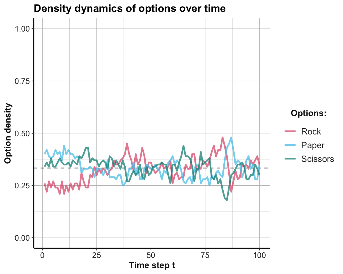
Interpretation
There is no evidence for any dominant strategy. As soon as one strategy is chosen more frequently than by chance, its opposite strategy becomes more successful. Thus, the population oscillates around the random baseline at \(p=1/3\), which is the optimal strategy in this competitive game with three symmetrical options.
- ad 4.: Here is the biased payoff matrix and some modified parameter settings:
# BIASED payoff matrices (per player) of the RPS game:
payoff_p1 <- matrix(c(1, 0, 4,
                      5, 1, 0,
                      0, 8, 1),
                    nrow = N_opt, byrow = TRUE)  # Player 1 payoffs
payoff_p2 <- matrix(c( 1, 0, 8,
                       1, 1, 0,
                       0, 2, 1),
                    nrow = N_opt, byrow = TRUE)  # Player 2 payoffs

# NEW simulation/agent parameters:
N_t <- 200       # number of games/rounds/time steps
epsilon <- 0.01  # exploration rate (epsilon-greedy model)

set.seed(468)    # reproducible randomness
To obtain the following result (shown in Figure 22.6), we reduced the model’s exploration rate epsilon to 0.01 (to obtain smoother curves) and increased the number of trials n_T to 200:
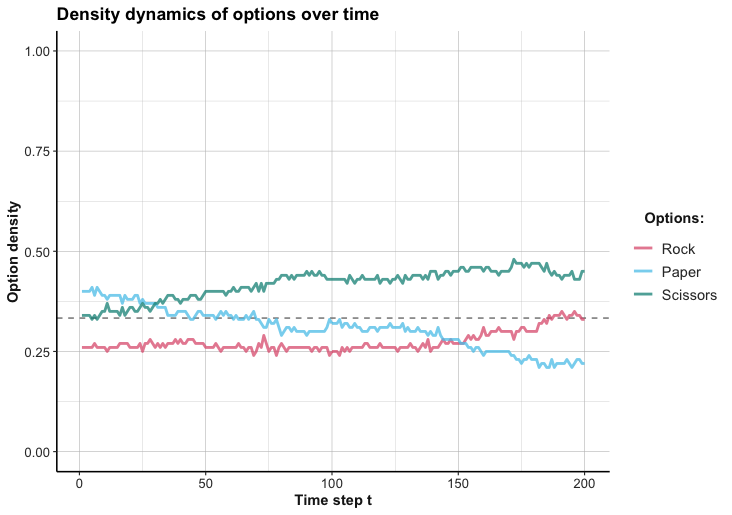
Figure 22.6: Density of option choices from 100 agents learning to play RPS with a biased payoff matrix.
Interpretation
It seems that the option with the highest payoff (i.e., “scissors”) is favored over the other options, but not by a wide margin. Interestingly, the second highest option (at the end of 200 trials) is “rock”. Winning with this option yields the least number of points, but it beats the popular “scissors” strategy. Overall, even the biased payoffs do not allow the population to gravitate toward a single strategy, as any strategy can be beaten by another.
22.6.5 Sequential mate search
A fundamental and important social game in the biological realm is provided by the problem of finding a mate to procreate. Mate search simulations are well-suited to illustrate the dynamics of social situations. However, they also contain many simplifying assumptions that may not hold in nature and society. In this exercise, we first create a basic simulation to explore some dynamics, before critically evaluating its results and deficits.
Assume a simulation for the following situation:
Assumption 1: Population:
Imagine a population of simple creatures: \(N_p = 200\) individuals, equally distributed into 2 types (i.e., \(N_p/2 = 100\) individuals per type), with procreation depending on a long-term hetero-sexual partnership.Assumption 2: Attractiveness:
All relevant features of an individual \(i\) for the this task can be summarized in its overall attractiveness score \(A_{i}\). As all individuals of the opposite type share the same criteria for evaluating attractiveness, an individual’s attractiveness for individuals of the other type are fully described by the rank of its attractiveness score (i.e., a value of 1–100, assuming no ties). However, the individuals of the population do initially not know their own attractiveness score and do not know the distribution of attractiveness values in the population (i.e., they initially do not know how many individuals with values above 50 exist).Assumption 3: Dating and marrying:
Two individuals of opposite types meet in a random fashion in a series of \(N_t = 100\) rounds of “dating”. In each round, the two individuals evaluate each other (based on some strategy that is only known to each individual) and decide whether they want to partner up with their match and make an offer if they do. Given a mutual choice for each other, the couple is matched (“married”) and removed from any further rounds of dating (i.e., married couples stay together).Assumption 4: Offspring and relationship value:
In each round after their marriage, a married couple produces an individual offspring with a probability \(P_{off}=.10\). As the attractiveness value of this offspring is the average of its parents, the value of a relationship can be summarized by \(N_{off} \cdot \frac{A_{i} + A_{j}}{2}\), where \(A_{i}\) and \(A_{j}\) are the attractiveness values of the married partners and \(N_{off}\) is the total number of a couple’s offspring.
-
Your task is to devise a successful strategy for 1/3 (34%) of each type of the population in an environment in which two other strategies exist (and are randomly distributed over all individuals):
1/3 (33%) of the population (of each type) follows an experience-based aspiration level strategy that wants to partner up with any date that exceeds the average attractiveness of the first 10 dates.
1/3 (33%) of the population (of each type) first aims to estimate their own attractiveness by monitoring the offers received on the first 20 dating rounds. They then estimate their own attractiveness (as the average of the attractiveness values of the partners who made positive offers up to this point) and then set their aspiration level to a partner that is at least as attractive as themselves.
Justify why you believe that your strategy is more successful than the other two.
- Create the simulation in R and evaluate the performance of all three strategies (numerically and visually). Which measures (beyond each strategy’s overall value) is informative regarding the success of a strategy?
Solution
General simulation parameters:
N_p <- 200      # population size
A_1 <- 1:N_p/2  # attractiveness ranks of type 1
A_2 <- 1:N_p/2  # attractiveness ranks of type 2
N_t <- 100      # number of time steps/trials/rounds
Note that the assumed value of a relationship can be directly computed when a match is made (at \(t_{match}\)) and is a linear function of \(P_{off}\), the remaining time periods (\(N_{t} - t_{match}\)), and the attractiveness values of both partners (\(A_i + A_j\)):
match_value <- function(t_match, p_off, A_1, A_2){

  t_left <- N_t - (t_match + 1)  # time left

  N_off <- p_off * t_left  # expected number of offspring in time left

  A_mean <- (A_1 + A_2)/2  # mean attractiveness of partners

  N_off * A_mean

}- Discuss in which ways these assumptions are not valid for human societies (which ones?), how more realistic assumptions would change the corresponding simulation, and what this means for the results from corresponding models.
Solution
There are many simplifying assumptions that clearly — and fortunately — do not apply to a realistic population of human beings. For instance:
- Each individual is assumed to belong to one of two types and assumed to seek an exclusive and stable relationship with an individual of the opposite type. Thus, both the population setup and the dating regime disregard the possibility of other genders, non-permanent relationships, and any non hetero-sexual preferences. Similarly, individuals who do not seek a relationship or remain childless are not accounted for and even discounted as worthless by the assumed value function.
Thus, the presence of superficial analogies in structure, process, and terminology (e.g., “attractiveness”, “dating”, “marriage”, etc.) must not trick us into assuming that this model reflects something fundamental about human societies. Essentially, the results of any simulation are only as valid as its assumptions — and we should at least be skeptical when a model makes many unrealistic ones.
Note, however, that we also emphasized that all models are wrong, but may still be useful (in Section 19.1). Thus, reasons for skepticism do not automatically render all model results useless. An advocate of this particular model could claim that it may fail for human societies, but may still mimick important aspects of some animal population. But beyond the flaws that may be fatal for depicting a human society, there are more subtle deficits that may also be violated by most animal organisms. For instance:
All individuals (in the population and within both types) are assumed to share the same preferences.
The assumption that individuals’ strategies are independent of their attractiveness score (due to being distributed randomly) is unrealistic.
An individual’s attractiveness score is an abstraction that serves multiple functions. First, it matters crucially for finding a match, then plays no role in the probability of procreation, but determines the value of a match again.
The round value \(t\) paces the dating regime (i.e., meeting one condidate per round), but also the rate of procreation (and thus the overall value of a partnership). In most animal populations, both time scales would differ from each other and not all individuals may follow the same rate.
Allowing for non-permanent relationships and extra-marital affairs could completely change the dynamics of the situation.
Thus, the simulation may be suited to illustrate some dynamics of social situations, but provides no realistic model of mate search in most human or non-human societies. Interestingly, if we re-frame the two types in terms of supply and demand (i.e., as repeated interactions between sellers and buyers) many people may be less critical and willing to consider the same simulation as a decent economic model of market interactions…
22.6.6 100 prisoners / boxes / numbers
Watch the following video (on the Veritasium channel) for an amazing problem and its analytical solution:
Now write R code that simulates the problem, and contrasts the performances of a random baseline strategy with the solution strategy.
Note
Implementing a known solution does not really require any social interactions between agents. But the problem was simply too fascinating to not mention it here.
See this blog post by Nathaniel Phillips for an elegant solution (involving functional programming with purrr).
As a teenager, I once recruited a friend to play the game to its alleged end after its 256th level. Although we tried hard to stay alive and awake, we never made it to the end.↩︎
Interestingly, prevailing scientific trends bias us towards immediately asking about the dog’s brain, rather than its auditory and olfactory senses, its digestive processes, or the nutritional or macrobiotic properties of its food.↩︎
The list of “other things” that are assumed to be equal here is pretty long (e.g., including some stability in options and preferences).↩︎
Social learning