3.2 RStudio Set-Up

Now that we have the proper applications downloaded to our computer, we can begin setting up our work space. As data scientists, we must keep our files organized. Ideally, your files are already organized in folders and subfolders. If not, you’ll find yourself adopting this practice soon enough (at least when dealing with R).

3.2.1 Creating a New Project

What is a Project?

A Project is essentially a folder on your computer. Like any other folder, a Project folder organizes files that you deem are related in one location. This location is called a working directory (WD). An example of a WD might look like this:

“/Users/Wendy/Documents/R Files”

Translated, the WD above tells us that we are currently working in the folder named: “R Files”. The rest of the information gives us information about the file path to the current WD. The “R Files” folder is located within the “Documents” folder. The “Documents” folder is located within a folder called “wendy”, which is located inside a folder called “Users”. What’s the difference between a working directory and a file path? All working directories are file paths, but not all file paths are working directory. A file path is an umbrella term that simply refers to a file location (all files have a file path just like every location on earth has a longitude and lattitude). A working directory simply specifies the file path we want to use now.

Like other folders, you should think about what you want your Project to contain. For example, I have different R Projects for different purposes. One R project contains all of the files (Word, Excel, R files, etc.) for my experimental study about nicotine reward. One R project contains files from my Summer 2019 R course. Another project contains files from my Intro Statistics course. You get the point. For now, let’s create an R project specifically for working on this book.

How to Create a New Project:

Upon opening RStudio (no need to open regular R Statistics), your screen should look like Figure 3.4.

You’ll notice that the console tells you which R version you currently have. By the time you read this guide, the version will have updated far past 3.5.2 (2018-12-28) – “Eggshell Igloo”, but that is my current R Statistics version.

It is important to periodically check R’s website to make sure that you update R Statistics to the latest version. You don’t need to download every R Statistics update, but there is a chance that some parts of your code will stop working if you wait too long. To update your R version, you will need to only download the new R Statistics, you do not have to download RStudio again.

Briefly, let’s check where our current working directory is located by typing getwd() in the console.

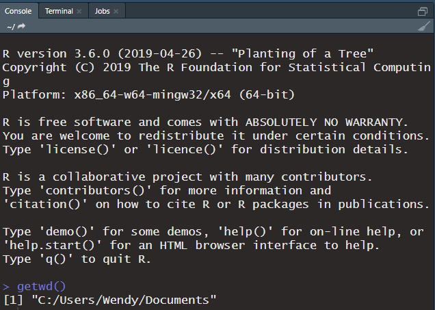
Figure 3.5: Executing ‘getwd()’ in the console to obtain the current working directory.

In Figure 3.5, we see that R is currently working and pulling information from my “Documents” folder. That means that when I save files, R will automatically save them to this folder. It also means that when I import files, they must be located within this folder. Check out the Files tab located on the lower right panel of R Studio. You’ll see all of the files/folders that are located in your current WD. When we create our new Project, you’ll see that the current WD will change.

Step 1:

At the top right corner of your screen, click on Project: (None) followed by New Project…. See Figure 3.6.

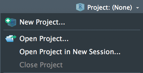
Figure 3.6: Creating a new project.

Step 2:

Click on New Directory > New Project. See Figure 3.7

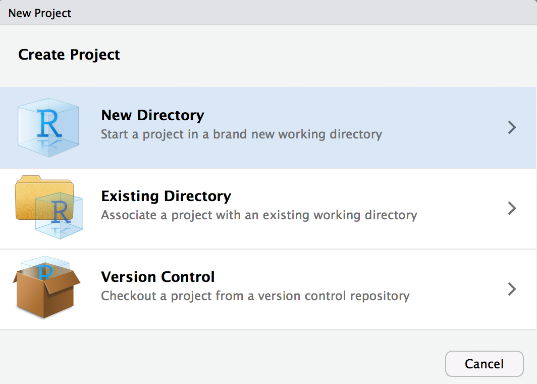
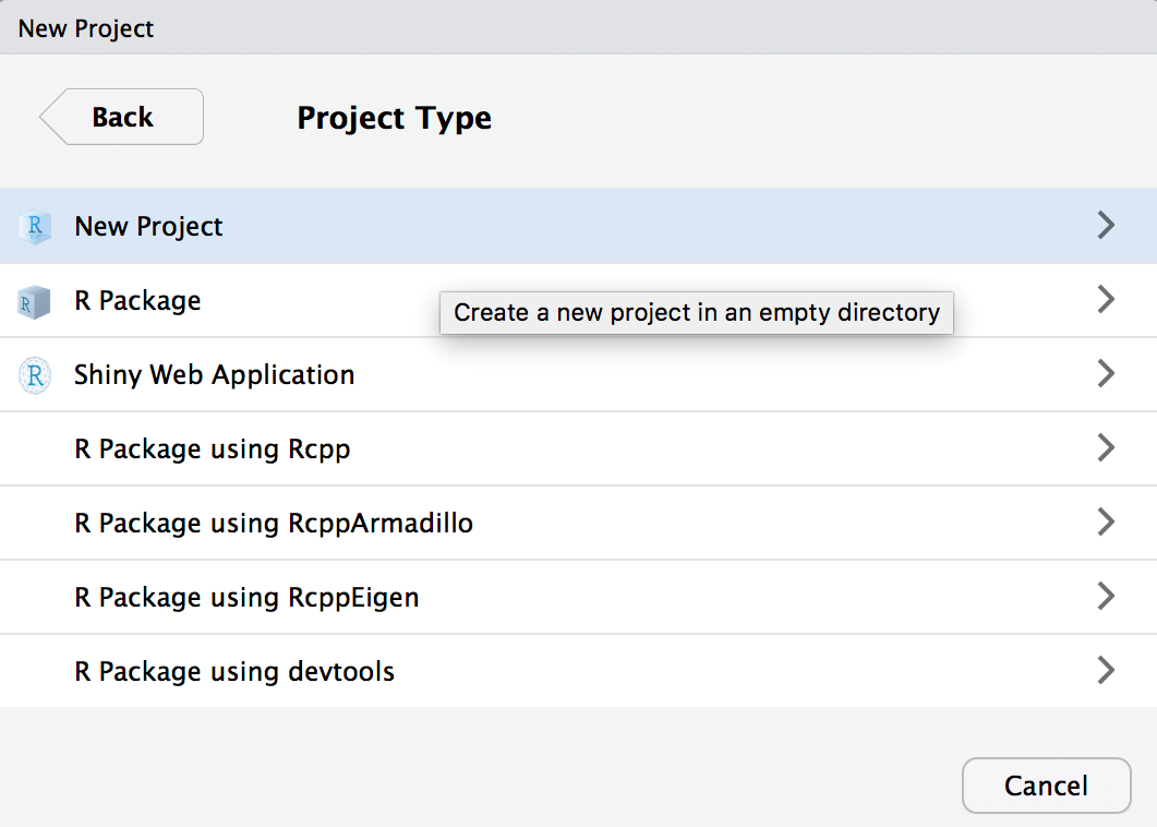
Figure 3.7: Creating a new project.

Step 3:

Name your folder. Here, I’ve named mine R Guide. See Figure 3.8.

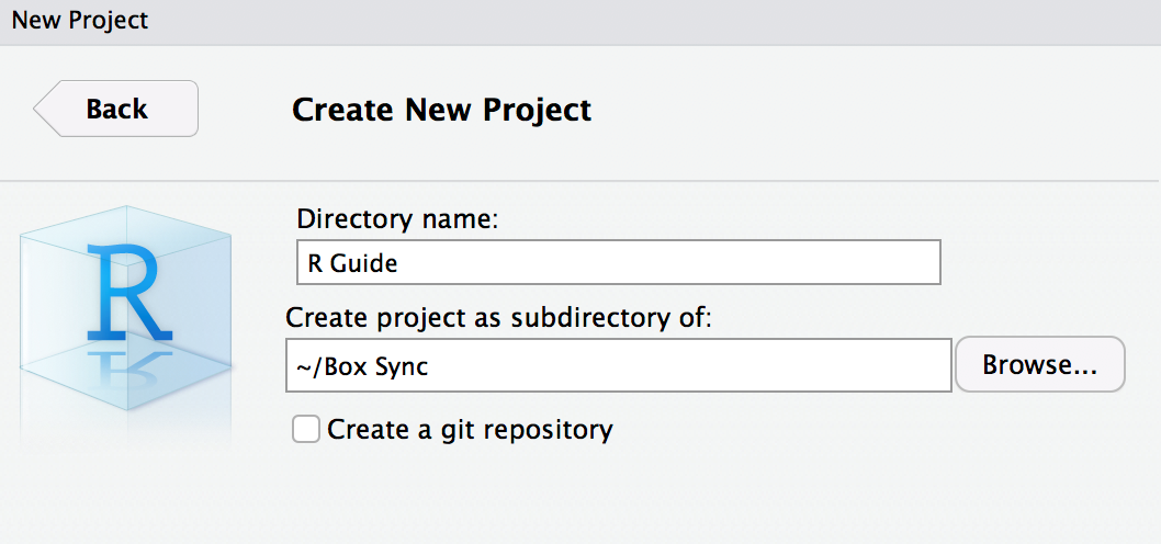
Figure 3.8: Creating a new project.

Step 4:

Under Create project as subdirectory of:, click on Browse…. Highlight (by selecting) the folder for which to create the Project folder and click Open followed by Create Project. In the example below, I have highlighted the folder “Guide to R”. This means my project folder will go inside “Guide to R”. See Figure 3.9.

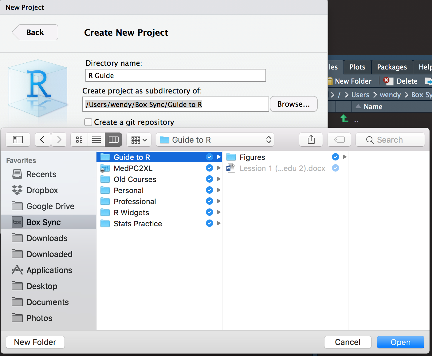
Figure 3.9: Setting up the directory for the project.

3.2.1.1 Checking the Set-up

In the top right corner of RStudio, you should now see the name of your project. See image 3.10.

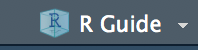
Figure 3.10: The project name is now displayed.

Let’s check your File Explorer (Windows) or Finder (MAC) to see how the folder is organized. See image 3.11.

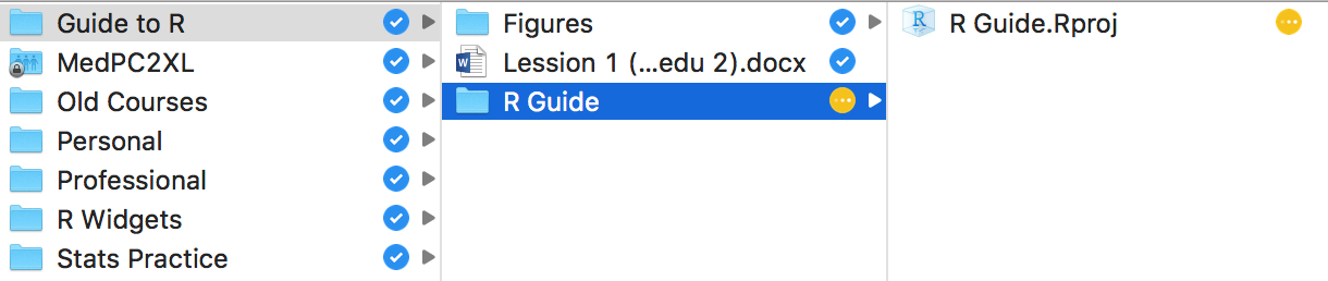
Figure 3.11: Checking the file location of the project.

My R project folder, named R Guide was created inside my Guide to R folder”. Inside the R Guide folder, R has created an .Rproj file. You can access this R Project any time simply by opening this .Rproj file. Directly opening the .Rproj file is my preferred method to open RStudio, but you could also choose to open RStudio from your desktop (clicking on the icon) and manually open the project by clicking on the drop down menu on the top right of RStudio. See Figure 3.12.

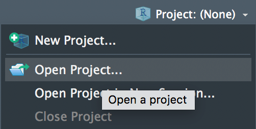
Figure 3.12: Alternative option of opening an R project.

If we execute getwd() again at this time, we’ll see that our current wd is set to our Project folder!

3.2.2 Creating a Script

Now that we have a project set up specifically for this guide, let’s create a script by clicking on the top left icon with the green plus sign or with the Shift + Control + N keyboard shortcut (Figure 3.13. A script is similar to a text document (e.g., Microsoft Word, Notepad, TextEdit, etc.) We can save our coding progress using a script and open it up later. Most of our code will be executed using the script. Many people create separate scripts for different purposes. For example, for every lab experiment, I have a script that organizes the raw data, a script that graphs data, and a script that performs statistical analyses. If you are unsure whether or not to create a new script, ask whether it would make sense to create a new Microsoft Word document for a similar situation. My recommendation is to create a new script for each chapter or significantly long section in this book. We’ll delve more into more detail in later sections.

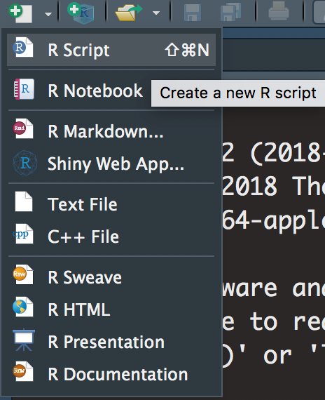
Figure 3.13: Create a new script.

Begin by typing a comment (i.e., text that is not recognized as code by R) by typing a # before the text: This is my new script! Then, save the script (Figure 3.14. This script will automatically save in the project folder (i.e., the current working directory). I do not recommend saving anything outside of this project folder at this time – more on this later. Here, I’ve saved my script under the name, “Script1”. You can choose to label your script with a more descriptive label or keep it simple.

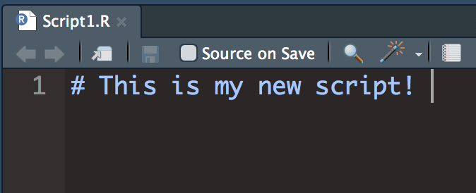
Figure 3.14: Save the script.

3.2.3 Installing Packages

Next, we will go over how to install R packages. R packages contain a collection of tools that allow R to perform certain tasks. For example, some packages are designed to help you graph while others help perform statistics. R packages can provide better ways to code in R by building on the foundational “base” code R has by default.

R packages only need to be installed once on a computer. The only times you would re-install a package is if you updated the R Statistics version (or for package updates). Just as new versions of software can slow down or not work on an older computer, updated packages may not work on an old R Statistics version. Similarly, a new computer (R versions) may not be able to run old software (packages), so it’s important that both the R version and the package version can work together. Remember that everything in RStudio is local to your computer. That is, if you want to use packages on multiple computers, you must separately install them for each computer.

For this guide, you will need to install the following packages: tidyverse, afex, emmeans, writexl, readxl, and ggthemes. In further sections, you may be asked to install additional packages, but these will give you a good starting point. Here is the code you will need to execute:

Notice that the names of the packages are surrounded by quotation marks!

Below are brief descriptions of how I will use these packages:

Name	Purpose
tidyverse	This package is actually comprised of multiple packages. The functionality is broad and useful. Its utility in my case lies in its abilities in graphing (ggplot2) and user-friendly formatting (dplyr). Installing this package will take some time—wait until the console is completely finished installing the package.
afex	I use this for statistics, particularly for ANOVAs (analysis of variance)
emmeans	This is another stats package. I use this for calculating the estimated marginal means for post-hoc analyses.
writexl	This allows me to produce Excel files from my R data.
readxl	This allows me to load my Excel files into R.
ggthemes	This provides additional tools for managing graphing aesthetics.

I recommend that you inactivate the install.packages() code after it has been executed once (Figure 3.15. This is done by highlighting the relevant code and using Ctrl + Shift + C. Remember that packages only need to be installed once per computer (unless you update the R version (Section 3.2.5). If you execute install.packages() for a package R already has installed, there will be a pop-up asking to restart the R session. When this happens, you can click Cancel and inactivate or remove the relevant install.packages() code. I highly recommend keeping a separate script containing a list of packages installed and the purpose they serve. Here is an example for what that script might look like:

install.packages("tidyverse") # Used for coding style
install.packages("afex")      # Perform stats (ANOVAs)
install.packages("emmeans")   # Calculates estimated marginal means

# OR

install.packages(c("tidyverse", # Used for coding style
                   "afex",      # Perform stats (ANOVAs)
                   "emmeans"))  # Calculates estimated marginal means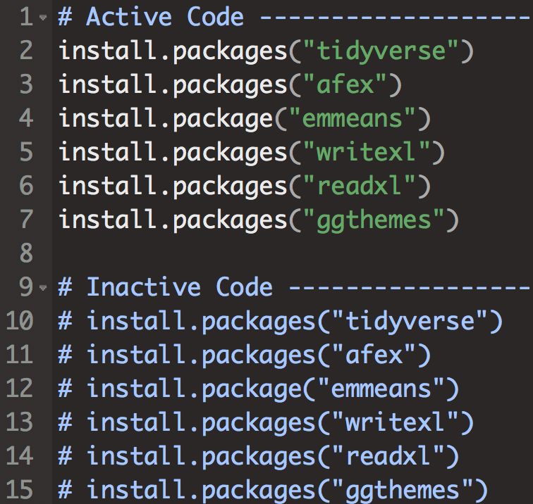

Figure 3.15: Inactivating install.packages() after use.

3.2.4 Loading Packages

Once packages are installed onto your computer, you must load them with library() each time you begin your R session (i.e., open up RStudio). Your installed packages are not automatically available to you upon the start of each session.

Begin by loading all of your libraries as such:

# The only necessary package for now.
library(tidyverse)

# These packages are not necessary to load at this point, 
# but it won't hurt to load them. Sometimes, packages may
# cancel each other out, so you may only want to load
# them when they are needed. However, these packages don't
# cancel out anything we need for this book. 
library(afex)
library(emmeans)
library(writexl)
library(readxl)
library(ggthemes)

Notice that unlike install.packages(), the name of the package in the library() function is not surrounded by quotations. These formatting details are unique and specific to the code. The more you practice R, the better you will be at recognizing these conventions.

These packages have far more utility available than what I will show you here. Packages are written by experienced R users who are looking to make their code more efficient and share their knowledge. There are far more packages available than I have ever used (currently almost 14,000!!; https://cran.r-project.org/web/packages/). How do you know which packages to use? I use these packages because many of the instructional guides and textbooks I’ve used also used them. Simply put – it’s all about word of mouth/internet posts that lead you to select a particular package.

You are now ready to follow along the examples and exercises. Don’t forget to periodically save your script just like you would a text document (Ctrl + S)!!

3.2.5 Updating the R Version

Periodically, you should update R. This must be done manually as R/RStudio will not automatically update the application. I typically update my R version about every three months. To determine what version you currently have, execute getRversion() in RStudio (be mindful of capitalization). Small version revisions are indicated by changes in the third digit whereas large revisions will change the middle number. There are a few ways to update your R version.

Computers running R on a Windows OS can easily update R through the original R application (i.e., R Graphical User Interface; GUI). See Figure 3.16. Using the R GUI application, execute install.packages("installr") followed by library(installr). Then, an “installr” tab will appear at the top of the screen next to the “Help” drop down menu. Under the “installr” tab, you can click on the “Update R” option. See https://www.r-statistics.com/2015/06/a-step-by-step-screenshots-tutorial-for-upgrading-r-on-windows/ for more information. Notice that there is an option to copy packages from the older version of R to the newer version of R. This eliminates the need to reinstall packages to the newer version of R.

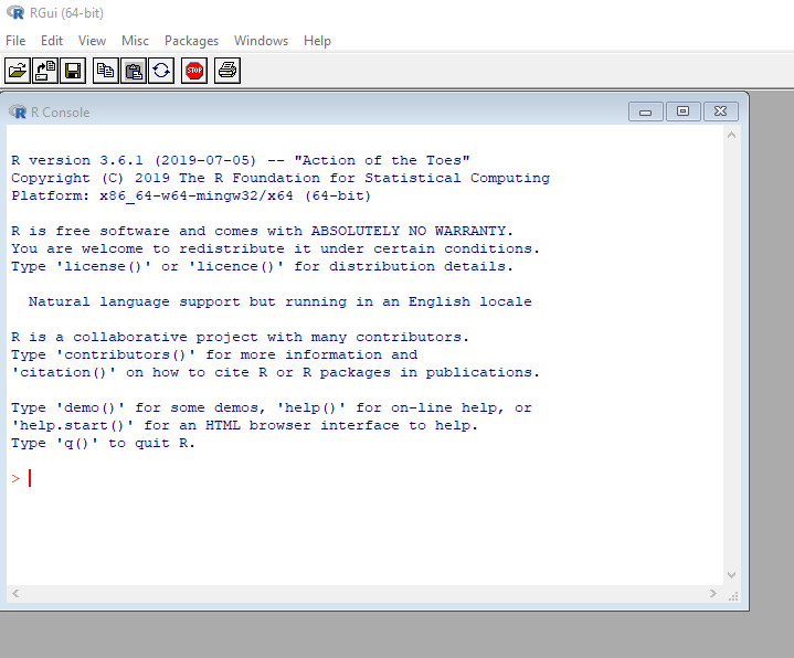
Figure 3.16: R GUI.

Alternatively, you can update the R version manually (any OS). This is procedurally identical to Section 3.1.1. This method requires packages to be reinstalled.