3.3 An Informational Tour
In this section, we will cover basic information (vocabulary/keyboard shortcuts) about R/RStudio.
3.3.1 Types of R Files
There are many different kinds of files that R can save. Here are the three common R-based files (require the R application to open) that we will encounter.
| File Type | Purpose |
|---|---|
| .Rproj | This is your project file in RStudio. This automatically sets your working directory to this containing folder. |
| .R | This is your script file. It contains your previously saved code. Like a Word Document. |
| .RHistory | R keeps track of all the commands you use in a session. |
3.3.2 Hot Keys to Remember
These are immensely useful shortcuts that will save you some time while coding. I highly recommend taking the time to practice using these hot keys. Some hot keys can use left or right arrows. Ctrl is short for the “Control” key.
| Commands | Function |
|---|---|
| Ctrl + Enter | Executes/runs code |
| Ctrl + Shift + C | Turns the current line of code into a comment. Inactivated lines will not be read and executed as normal code. |
| Ctrl + Left/Right Arrow | Moves your cursor all the way to the right/left |
| Ctrl + Shift + Left/Right Arrow | Highlights entire line to the left/right of your cursor |
| Alt + Left/Right Arrow | Moves your cursor one chunk of letters at a time |
| Alt + Shift + Left/Right Arrow | Highlights one chunk of letters at a time |
| Ctrl + A | Select all text |
| Ctrl + S | Saves the file. Do this every few minutes to save your progress. |
| Ctrl + Shift + R | Creates headers for your R script. You can easily navigate between labeled sections of your R script. |
| Ctrl + Shift + M | Shortcut for %>%, also known as a “pipe”. The pipe symbol is frequently used in the tidyverse-style syntax. More on pipes later. |
| Alt + Shift + K | Displays all programmed keyboard shortcuts for R. |
3.3.3 Executing Code
To execute (AKA run or evaluate) code in R, you must place your cursor (blinking vertical line) on the line of code for which you want to execute. You may place your cursor at the beginning, middle, or end of the line – the placement doesn’t matter since R will execute the entire line. See Figure 3.17.
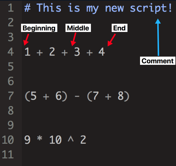
Figure 3.17: Your cursor can be placed anywhere on the line when executing code. Note that comments are not recognized by R as executable code.
After you have placed your cursor in the proper line, use Control + Enter (Ctrl + Enter) to execute the code. If you are using a Mac, you may also use Command + Enter (Cmd + Enter) – the end result is the same.
3.3.3.1 Exercises
Use a script to type and execute code in the following exercises (see Section 3.2.2 for information on creating scripts).
- Type out the following code in your script (including comments):
# This is a comment!

## Problem A (also a comment)
1 + 2 + 3 + 4

## Problem B (hit 'Enter' after the plus sign before '4')
1 + 2 + 3 +
  4

## Problem C
9 * 10 ^ 2- Notice that R automatically indented
4when you hit Enter after1 + 2 + 3 +. This is because R recognizes that you are not finished coding this line. A plus sign indicates that there will be another item to add. Even though1 + 2 + 3 +and4are on separate rows, R still considers this as one continuous line of code; thus, you may place your cursor anywhere on this continuous line of code to execute it (top row/bottom row). Many programmers prefer to add these stylistic breaks in code to aid in visual aesthetics. That is, pressing Enter after specific punctuation marks (,,+,%>%) to introduce breaks will make code easier to read without the need for horizontal scrolling. Practice typing code with and without breaks in these examples:
# No breaks
(1 + 2 + 3) + (4 + 5 + 6) + (7 + 8 + 9) + (10 + 11 + 12) + (13 + 14 + 15) + (16 + 17 + 18)

# Includes breaks
(1 + 2 + 3) +
  (4 + 5 + 6) + ## notice the indentation after the first line
  (7 + 8 + 9) +
  (10 + 11 + 12) +
  (13 + 14 + 15) +
  (16 + 17 + 18)
Place your cursor at the top of Exercise #1 (on the same line as the comment). Begin executing code (Ctrl + Enter), repeating this after each line is executed. Each time you execute a line of code:
There is an output shown in the console. This output is the result of the code evaluation.
The cursor automatically moves to the next line of text, whether it’s a comment or active code. You do not need to manually move the cursor to the next line of code!
Comments are not executed as code.
After you run out of code to execute, the console will produce empty prompts (
>) without outputs if you continue to press Ctrl + Enter.
You can also execute code by selectively highlighting the text. For this exercise, highlight the code in the example below one line at a time and execute them. Make sure that
+is not the last character you highlight! You wouldn’t end a sentence with a comma, so don’t execute code that’s not finished (i.e., ends on a comma (,), plus sign (+), or pipe (%>%))!
1 + 2 + 3 # highlight and execute '1 + 2 + 3' without this comment!

1 + 5 + 7 # highlight only '1 + 5' and execute- You can also choose to execute all of the code in your script. The easiest way to do this is with Ctrl + A followed by Ctrl + Enter.
3.3.4 Typing in the Script versus the console
There are two panes in R Studio where you can execute code: in the script or in the console. The script is an archivable file (i.e., can be saved to a file on your computer) whereas the console is (generally) a temporary space to execute code. Executing code in either space will produce the same output; however, programmers use scripts to save their progress for later use.
So why would you ever execute code in the console, a space that won’t save what you’re doing? As a beginner, you probably won’t do this often because you need to familiarize yourself with the code; you’ll likely need to come back to a saved script to remember which code performs which task. As you become proficient in R, you may not want to save every single detail in a script. Perhaps you’d like to test out a chunk of code. Scripts are like Microsoft Word/text documents. Sure, you could rewrite all of your code each time you opened RStudio, but that would be like re-writing your essay assignment each time you opened Microsoft Word. In contrast, executing code in the console is more like typing in URLs in a web browser. You usually do not need to save short URLs once you’re familiar with them (e.g., who needs to bookmark Google.com?).
3.3.4.1 Exercises
Let’s get more practice executing code.
- Type out the following code in your script:
# This is a comment
# Comments don't get evaluated as code by R.

## Problem #1
1 + 2 + 3 # sum of 1, 2, and 3

## Problem #2
1 - 2 - 3 # difference of 1, 2, then 3

## Problem #3
"hello"

## Problem #4
# 4 + 5 + 7

## Problem #5
# hello
Execute all of the above code with Ctrl + A followed by Ctrl + Enter.
Notice how R did not evaluate
4 + 5 + 7in the console like in Problem #1 and Problem #2. This is because4 + 5 + 7is a comment! There is a # symbol preceding the addition problem.Execute one line at a time by repeatedly pressing Ctrl + Enter
Execute each Problem in the console.
Notice that the console will execute text using Enter whereas the script requires Ctrl + Enter. It is also slightly less visually pleasing to execute lengthy code in the console. We cannot easily insert breaks for styling purposes.
Highlight and activate
# 4 + 5 + 7(Ctrl + Shift + C)Notice how the # symbol disappeared. This highlighted portion can be inactivated again with Ctrl + Shift + C. I refer to certain comments as inactivated code. That is, if these comments were activated, they would produce an output.
Place your cursor between the
2and+in Problem #1 and execute.Place your cursor at the end of Problem #1 (after
3) and execute.Place your cursor at the beginning of Problem #1 (before
1) and inactivate the line.Notice how the rules for inactivating a line of code is similar to executing the line. You may choose to inactivate code via highlighting specific lines. Inactivating via Ctrl + Shift + C inactivates the entire line. To inactivate a portion of the line,
#must be placed manually.Highlight
1 + 2in Problem #1 and execute.Notice that only the code in this highlighted portion is executed. That is, R only added
1 + 2and excluded+ 3despite its presence in the script. R will ignore all text/code outside of the highlight when using this code execution technique.Highlight
2 + 3in Problem #1 and execute.Highlight
1 + 2 +in Problem #1 and execute.Notice that nothing appeared in the console. R is waiting for additional code. Since the code ended with a
+, R is waiting for you to enter in additional code. This particular code portion could be read as:“1 adds to 2 adds to…”
You essentially didn’t finish the sentence! To exit out of this incomplete code, place your cursor in the console and hit ESC on your keyboard. When you see
>in the console again, R is ready to try again. If you forget to hit ESC and reset the console input, you will likely encounter an error.Inactivate Problem #5’s code with Ctrl + Shift + C,
# hello, and execute the codehello.Notice that you’ll get an error that reads:
Error: object 'hello' not found. This is because R recognizes letters in a few ways:As values/definitions
As an object
If letters/words are values, you must place the word(s) in between quotations such as in Problem # 3. If letters/words are objects, they must be explicitly defined in the environment by the user. In this example, R expects
helloto be an object (and not a value) because it is not enclosed by quotation marks. More on objects in the next section.The console holds a limited memory for recently executed code. Now that you’ve executed some code in RStudio, click in the console pane and press the “up” arrow on your keyboard. This is a quick and simple method to re-execute a line of code.
3.3.5 Vocabulary Terms
In this section, we will go over some of the common terms used in R. These are the vocabulary terms that we have seen so far:
| Vocabulary Term | Definition |
|---|---|
| R Statistics/R | “R” can refer to the R Statistics application or to R as a language. |
| Base R | Base R refers to the coding tools available by default in R. It is frequently used to describe the default coding style/rules (i.e., base R syntax). Base R packages and functions are always automatically loaded upon opening RStudio. Many R users use additional packages that utilize Base R code as a foundation to produce more efficient/attractive code. The tidyverse syntax style, which builds from base R, is increasingly being adopted by the R community; however, there are situations where Base R is still preferred. |
| RStudio | This is the Integrated Development Environment (IDE) that facilitates R coding. Simply put, RStudio organizes R code in a user-friendly manner. R by itself is just the language whereas RStudio is the program that houses and uses the R language. The R language can be used without RStudio. However, RStudio is more organized, visually appealing, and powerful than the default R application alone. |
| Package | A collection of free R tools that an R User wrote. Anyone can create a package (with advanced R training). Packages were written to making tedious coding tasks more efficient. Different packages will provide different sets of tools (i.e., wrench set vs. screwdriver set), though some tools may have overlapping functions (i.e., scissors vs. knife). Packages are free but must be installed to your computer first. After installation, packages must be loaded into your RStudio library each time RStudio is opened/launched. |
| Script | Scripts provide a space to type, execute, and save your code. These saved scripts can be opened at a later time to edit or execute again. Upon each new RStudio session (i.e., every time you open RStudio), RStudio is a blank slate and you must re-execute your code. Scripts allow users to save previously written code so that re-executing code is simple. With RStudio, you can even open up multiple R Scripts in separate tabs. R Scripts are like Microsoft Word (or any text-editing application): both filetypes can save previous work/text so that the user does not need to re-type its contents and both can be opened on any computer with the application installed. |
| Console | This is a universal feature in R Statistics and RStudio that displays the output of executed code. That is, each time code is executed, the console will display the line(s) of code used and the outcome. Code can be executed directly through the console or indirectly through the script. Executing code in the console only requires you to hit Enter, while executing code in the script requires Ctrl/Cmd + Enter. Code that is executed in the console will not be saved to a file – it is best practices to use a script if you want to save code for later use. |
| Project | An organizational tool that sets up a designated location (i.e., folder) on the computer for the R user. Any file that is saved/exported by R will be saved in this designated location/folder and any file that is imported into R must also be located in this folder. |
| Working Directory (WD) |
This is path to the folder in which you are working. Computer files are located in specific folders and those folders are oftne nested inside other folders. For example, my photos from Christmas 2018 are located in a folder named Christmas. The file path to this folder is: “C:/Users/Wendy/Photos/Christmas” where each word in this path represents a folder. That is, I must open the C-drive on my computer, click on the Users folder, then Wendy folder, then Photos folder, and finally the Christmas folder to get to my Christmas 2018 photos. Setting this file path as my working directory would mean that I am setting the Christmas folder as my default folder for everything (i.e., for saving files or importing files). A working directory can be set to a specific file path manually (via coding) or it can be automatically set using an R Project. The working directory in an R Project will always be the file path to the .RProj file by default.
|
3.3.6 The Global Environment
This is the “work-space” in which your code is working in. You always want to start your R session with a clean environment (i.e., no objects defined; see 3.18). To clean out your environment, click on the broomstick icon in the Environment panel.
The Environment is where objects are temporarily saved for the duration of your R session; the session is over when you have exited RStudio. Objects are things you have defined (e.g., values, datasets, graphs, functions) within your R script. You can refer back to the object at a later time for when you need it again.
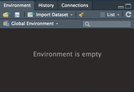
Figure 3.18: Empty environment.
3.3.7 Using Objects
Saving information to objects in the environment is useful to cut down on the amount of coding. Think back to algebra class where you had to solve for “x”.
If x + 4 = 10, we know that x = 6. That is, x is an object defined as the value of 6. Now that we have a definition for “x”, we can use this object in place of 6. x + 20 would represent 6 + 20.
In R, we can define objects using the <- operator. Notice how the object appears in the Global Environment after it is defined (via code execution; Ctrl + Enter).
x <- 6We could also create objects with more complex definitions. c() is a function that allows R to concatenate or group together the contents listed inside the function.
y <- c(1,2,3,4,5)…and choose more complex object names (single letter names are frowned upon).
numbers <- c(1,2,3,4,5)We can perform tasks on complex objects as we’ve done before with simply defined objects.
mean(numbers) # calculates the mean of values in the object## [1] 3numbers + 1 # adds 1 to each number in the object## [1] 2 3 4 5 6sum(numbers) # calculates the sum of values in the object## [1] 15…and we can define these tasks as objects as well! Remember that the object name is determined by us (although there are limitations to usable names as we’ll see later in Section 3.4.2)!
numbers.mean <- mean(numbers)
numbers.add1 <- numbers + 1
numbers.sum <- sum(numbers)
You can also define entire datasets as objects! The possibilities are endless.
It’s important to note that you can only use the object if it has been defined in the Global Environment. Objects should only remain defined within the current RStudio session (a caveat to this will be discussed in 3.5). Once RStudio is closed out on your computer, the objects must be redefined the next time RStudio is opened. Always start with a clean environment each RStudio session. This is where scripts come in handy. Rather than typing out the definitions for every object upon a new RStudio session, you can save a script that contains the code! Code that is saved to a script can then be executed any time.
3.3.7.1 Practice with Defining Objects
First, let’s make sure that our environment is completely empty (see Figure 3.18). To empty out the environment manually, click on the broomstick icon and confirm that all objects are to be removed from the environment. Go ahead and check “Include hidden objects” as well. Make sure that you have a script created (see Section 3.2.2 for how to create a script)!
Now, let’s dive into some exercises:
- Execute the following code to create 5 objects in the environment:
# creating an object named "student.names" that contains three names
student.names <- c("Matt", "Remi", "Wendy", "Craig")

# creating an object named "fav.color"
fav.color <- c("red", "purple", "teal", "yellow")

# creating an object named "age"
age <- c(29, 2, 24, 15)

# height in centimeters
height <- c(177.8, 38.1, 170.18, 30.48)

# human or cat?
species <- c("human", "cat", "human", "cat")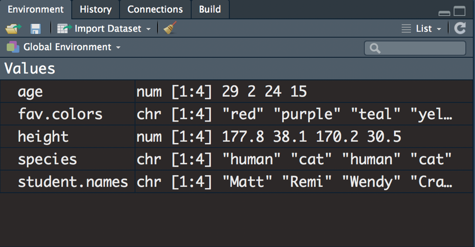
Figure 3.19: Environment with 5 objects.
- Next, let’s combine these objects into a single dataset:
data <- tibble(student.names, fav.color, age, height, species)- Execute
datausing one of methods discussed in 3.3.3. Your console output will look like this:
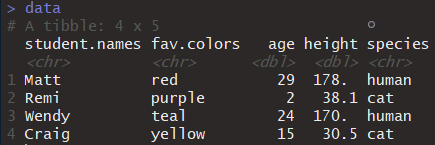
Figure 3.20: Console output after executing the data object.
- You can also view your
dataobject in a separate RStudio tab. This can be done by clicking on thedataobject in the Environment or by executingView(data):
Figure 3.21: Object named ‘data’ in the global environment.
Ultimately, this is the result:
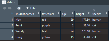
Figure 3.22: View of object named ‘data’.
3.3.8 What is a Function?
Functions are a useful tool that allows you to perform tasks quickly and efficiently. Quite frankly, they are the backbone of any R code. I often get asked how I know the names of the functions that I use, and the short answer is: through Google and practice. There are functions I happen to use a lot in my code and through repeated usage, I have come to memorize what functions I need for the situation. Just like learning when you should use a screwdriver versus a hammer versus glue for a crafting project, you learn which tools are appropriate through repeated use.
All of the functions I utilize were ones that various guides and tutorials used to accomplish a specific task. These functions were all written by someone else, who defined how the function should work. At this time, you will not need to learn how to write your own functions. Many people don’t ever write their own functions because all of their coding needs are satisfied by what is currently available. Despite this, learning how to write functions (after you’ve got the basics down) adds another layer of knowledge that could be useful for more complex coding in the future.
3.3.8.1 The Anatomy of a Function
The anatomy of a function is structured into two main parts: the name and the arguments. The name of the function is listed on the left side of the parentheses while the arguments are located inside the parentheses: name.of.function(argument1, argument2).
Some examples of functions include:
library()ggplot()mean()
You can look up a function’s help page by executing a question mark before the name of the function as such:
?library?ggplot?mean
Here, the mean function has one mandatory argument labeled x. Here, x is defined as “an R object”. The mean() function also has some built-in optional arguments that may be useful in certain circumstances. The second argument for the mean function is trim and the third argument is na.rm. The na.rm argument is particularly useful if your object contains a missing (NA) value. The na in na.rm stands for NA and rm stands for remove. Under default settings, using the mean function on an object with NA values will result in a NA output because this function does not remove NA values before performing its operations.
3.3.8.2 The Function of a Function
Arguments are the objects that functions use. For example, if you wanted to use a hammer as your tool, you want to know what object to use the hammer on (i.e., bird house). If you don’t specify which object you need to use your hammer on, the hammer just sits there and does nothing. Similarly, if you don’t specify arguments within a function (mean()), nothing really happens.
Sometimes, you may need to know multiple pieces of information before you use the hammer. What kind of material is the bird house made of? How fragile is the material? How big is the bird house? Are there certain parts of the bird house where you can’t use the hammer? Similarly, some functions will need multiple arguments to work. Most functions also have optional arguments that aren’t usually necessary but can add extra specifics that might be useful aesthetically or peripherally.
Functions within Functions: Using Multiple Functions at Once Just like performing multiple operations on a graphing calculator, you can utilize many functions at one time by nesting them within each other. For example, you can choose to round the mean of an object to the nearest whole number as such:
round(mean(numbers2, na.rm = T), 0)Here, the round() function is used outside/around the inner mean() function that we have used so far. When we solved for the mean of numbers 2 previously while removing NAs, the result was 2.5. To round to the nearest whole number, we use the round() function. This function requires an object x and the number of digits argument that specifies how many digits to the right of the decimal to keep (see ?round for more information). Since we want the nearest whole number (i.e., no decimal points), the digits argument (second argument) is 0. It is possible to nest as many functions within themselves as you want; however, this can become difficult to keep track of which argument belongs to what function. One way to mediate some confusion is to determine which parenthesis belongs to which function. By moving your cursor to the right side of a parenthesis, R will automatically highlight the corresponding paired parenthesis. I should also mention that the second most common mistake in coding is to forget to add a closing parenthesis, leaving a lonely open parenthesis hanging. Not to worry—R will let you know of this issue by issuing an error message any time you are missing the proper punctuation/symbol.
3.3.8.3 Functions help with efficiency
Instead of calculating the mean of the numbers 1,2,3,4,5 like this:
# calculating the mean of numbers 1 through 5
(1 + 2 + 3 + 4 + 5)/5
## [1] 3You can do this faster with the mean() function
Method #1:
mean(1:5)

# The colon indicates "through" as in the mean of numbers 1 through 5
Method #2:
mean(1,2,3,4,5)

# typing all of the numbers manually as arguments for the mean function
Method #3:
Numbers <- c(1,2,3,4,5)
mean(Numbers)

# creating a separate object that contains the values for which to use
# in the mean() function. The object is defined as the concatenation of
# numbers 1,2,3,4,5 via the concatenation function, c()| Example | Code |
|---|---|
| This is a function I want to use. It calculates the mean of an object. |
mean()
|
| This is an object I created. The <- symbol indicates an object is being defined, where the object name is located on the left of the symbol and the definition is on the right. Here, Numbers is defined as the concatenated vector containing numbers 1 through 5. |
Numbers <- c(1,2,3,4,5)
|
If I want to calculate the mean of my object called Numbers, I would put Numbers as an argument within the function mean().
|
mean(Numbers)
|
But let’s say we’ve got a special object that contains a NA value.
|
Numbers2 <- c(1,2,3,4,5,NA)
|
Executing this would lead to a NA result. R will not be able to calculate the mean, because there is a missing (NA) value.
|
mean(Numbers2)
|
However, the mean function includes an optional argument that allows the function to ignore the NA value and continue to calculate the mean without it. Here, na.rm = TRUE (notice the capitalization required) specifies that mean() should remove (rm) all NA values (na) when calculating the mean of Numbers2. By default, na.rm = FALSE. In this case, you must manually switch na.rm to be TRUE. You can choose to include this second argument for Numbers object, but because there is no NA value, there is no change in consequence.
The default setting for these optional arguments is usually listed in the help page for each function (accessed by executing ?mean)
|
mean(Numbers, na.rm = TRUE)
|
3.3.8.4 Exercises
- Pull up the help pages for the following functions (hint: use a question mark):
library()ggplot()mean()
- Create two objects:
numbers <- c(1,2,3,4,5)
numbers2 <- c(1,2,3,4,NA)
You can view the definition of numbers and numbers2 any time by executing just the name of those objects:
numbers
numbers2
Notice that your Environment has also changed since you’ve defined these objects. Remember that in order for the Environment to save information, you must define it with the <- symbol (see Section 3.4.3 for more information about built-in symbols):
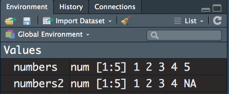
Figure 3.23: Defining numbers and numbers2.
Next, calculate the means of each object as such (what do you see?):
mean(x = numbers)
mean(x = numbers2)
Next, add the na.rm argument. Here, adding na.rm = TRUE is redundant, because the numbers object does not have any NAs to remove in the first place:
mean(x = numbers, na.rm = TRUE)
mean(x = numbers2, na.rm = TRUE)
Notice that TRUE turned a different color. Code that reads TRUE and FALSE are recognized by R as a special phrase. In shorthand, you could type T instead of TRUE and it would produce the same result. Similarly, F and FALSE mean the same thing:
mean(x = numbers, na.rm = T)
mean(x = numbers2, na.rm = T)
As you become familiar with functions, you can omit the argument name:
mean(numbers)
mean(numbers2)
This is because R assumes that the first argument entered into the function is the x argument. We can see the assumed order of arguments by viewing the function’s help page (see ?mean for the help page). If the first argument I entered in the mean() function was not the x argument, I would need to specify what argument the value belongs to:
mean(na.rm = T, x = numbers)
mean(na.rm = T, x = numbers2)
In the mean() function, the order that R expects to receive arguments is:
mean(x, trim, na.rm)Although we haven’t talked about the trim argument, it is technically listed as the second argument for the mean() function. Remember, x, trim, and na.rm are the names of the arguments—they are not the arguments themselves. As such, you do not have to include the argument names in the function as long as you remember the order in which the arguments must be listed. For example, you can omit the x argument label for the first argument:
mean(numbers, na.rm = TRUE)
# or
mean(numbers2, na.rm = T)
But you can’t run this:
mean(numbers, TRUE)
# or
mean(numbers2, T)
This is because na.rm is the third argument in the mean() function. Without the na.rm label specification, R is assuming that the second value that I enter is the trim argument (see ?mean for more information). Remember: although the R help page will specify many arguments available for a function, not all of them are mandatory (i.e., trim, na.rm). Some are required in some circumstances (i.e., na.rm = TRUE is necessary when the object x has a missing value). Some are never required and can be used to the user’s discretion (i.e., trim).
3.3.9 Pipe/Piping (%>%)
Pipes are a convenient tool to organize the tidyverse syntax style of coding. Recall that there are two major camps of coding syntax: tidyverse and Base R. Both have pros and cons and while most R users use a mix of the two, people typically favor one more. I personally prefer tidyverse when it’s feasible. To understand what a pipe does, we first need to understand some Base R syntax.
Recall that a dataset is a group of related variables. That is, each variable represents a column and each row represents a unique observation. Here is an example of a small dataset. Notice that each column represents a variable and each row represents a unique individual (animal).
## # A tibble: 4 x 3
##   Subject Animal CoatColor
##   <chr>   <chr>  <chr>
## 1 Craig   cat    brown
## 2 Aries   dog    black
## 3 Remi    cat    grey
## 4 Duke    dog    brown
Base R’s datasets are called data frames or df. This is how the data is structured in R by default. Tidyverse-styled datasets are called tibbles or tbl. Tibbles have all of the same properties as data frames and more. Tibbles are designed to be used with the tidyverse syntax style. Check out Table (()) for comparisons between data frames and tibbles.
Pipes are a shortcut tool (Ctrl + Shift + M) that the package known as tidyverse uses for more efficient coding and improved readability for the user. Hitting Enter after a pipe will auto-indent and organize your code in a readable manner.
Technically, the pipe is derived from the package magrittr specifically, but tidyverse loads magrittr (in addition to other packages) and thus contains the pipe operator.
For example, let’s say I want to create a new variable called Milliliters from a variable containing values from the variable Liters. I also want to create a new variable called Deciliters from Liters:
Base R:
df$Milliliters <- df$Liters*1000
df$Deciliters <- df$Liters*10
Read the above code as: I am defining Milliliters (as a new variable in
df) as Liters (obtained from a data object calleddf) multiplied by 1000. Then, I am defining Deciliters as (as a new variable indf) as Liters (obtained fromdf) multiplied by 10The dollar sign indicates that the word following the dollar is found within the word before the dollar sign.
Tidyverse R (using a tibble): You can choose to type this in one line:
df %>% mutate(Milliliters = Liters * 1000, Deciliters = Liters *10)Pressing Enter after certain kinds of punctuation (pipes and commas) auto-indents the code in a more readable manner:
df %>%
  mutate(Milliliters = Liters * 1000,
         Deciliters = Liters * 10)
Read the following code as:
“Within my data object, I want to mutate/change things by creating a variable called “Milliliters”. Milliliters is based on the currently available variable, Liters. Specifically, values of Milliliters should be Liters multiplied by 1000. I also want to make a new variable called “Deciliters” from Liters values multiplied by 10."
This example is a simple one and not very telling of how tibbles make things more efficient than base R but trust me when I say that using tibbles will reduce entry error in the long run.
3.3.10 Types of Data
There are many different structural types of data. That is, data can be numerical, letter characters, boolean (TRUE or FALSE values only), categorical, etc. We might refer to data as a single variable, but we could also have data that has multiple variables (i.e., dataset). In this section, we will discuss common types of data and when they are used/what they are used for.
3.3.10.1 What is a vector?
If you are unfamiliar with this term, it is a data structure which contains a single type of values (e.g., all letter characters or all numerical type). If you combine multiple vectors together, you can create a dataset. Each column within a dataset is a vector. On their own, each column in isolation simply gives us a bunch of values. Combining multiple vectors to form a dataset can paint a story of those values.
Let’s say we have:
One vector containing the Names for each subject
One vector containing the Hair color for each subject
One vector containing Age for each subject
One vector containing a TRUE/FALSE value called Human
When you look at each individual vector separately, it’s just a list of numbers/words. If you put all three vectors together, you can create a dataset. Datasets imply some order to rows AND columns. Let’s see an example.
Let’s say that:
Sam has brown hair and is 24 years old and is a human.
Tina has black hair and is 41 years old and is a rabbit.
Alex has blonde hair and is 2 years old and is a human.
We must ensure that each piece of information remains with the relevant person; thus, the order for each vector’s values will matter when we put the vectors together. For example, all values related to Sam must be arranged first in each vector.
## Defining three objects, all of which are vectors
# A vector containing "Names"
Names <- c("Sam", "Tina", "Alex")

# A vector containing character values representing "Hair Color"
Hair <- c("Brown", "Black", "Blonde")

# A vector containing numeric values representing "Age"
Age <- c(24, 41, 2)

# A vector containing TRUE/FALSE (T/F) values representing human/not human
Human <- c(TRUE, FALSE, TRUE)

## Executing three lines of code to view these objects' definitions in the console
Names
Hair
Age
Human

## Defining an object named mydataset
# This dataset that combines the four vectors defined previously
mydataset <- tibble(Names, Hair, Age, Human)

## Viewing the dataset in the console
mydataset
## # A tibble: 3 x 4
## Names Hair Age Human
## <chr> <chr> <dbl> <lgl>
## 1 Sam Brown 24 TRUE
## 2 Tina Black 41 FALSE
## 3 Alex Blonde 2 TRUE3.3.10.2 Atomic Vector Types
Each vector can be categorized based on the types of values it contains. There are five basic types of atomic vectors.
| Atomic Vector Types | Examples |
|---|---|
| Character (AKA a string) | “a”, “labels here”, “can be a combination of any letters, numbers, and symbols.” |
| Numeric | 2, 15.5 |
| Integer | 2L (L tells R to store this value as an integer) |
| Logical | TRUE or T, FALSE or F (in all capital letters) |
| Complex | 1 + 4i (complex numbers with real and imaginary values |
R has a hierarchy of data structures where certain atomic vector types are “more specialized” than others.
The order of least specialized to most: character, numeric, integer, logical, complex
R will default to the least specialized it can get unless you specify otherwise
If your values contain any letters, variable will default to the character structure.
If your value only contains numbers, the variable will default to the numeric structure
Values for a variable with an integer structure must be real and whole numbers
Values for a variable with a logical structure can only be
TRUEorFALSE
You can use str() to view the structure types for all of the variables in your dataset.
Example
Compared to built-in mtcars dataset, which only has numeric variables, some variables in the diamonds dataset are numeric, some are ordered factors (ranked categories), and one is an integer. In my color scheme, purple text indicates code that has been executed in the console. White text shows the result of the executed code.
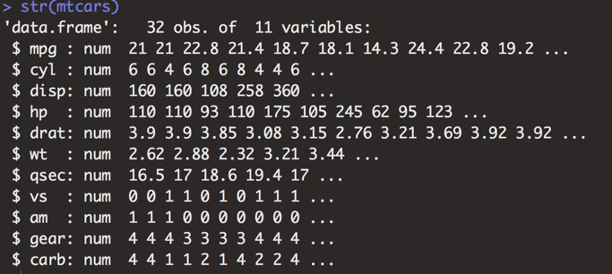
Figure 3.24: Data structure of the mtcars dataset.
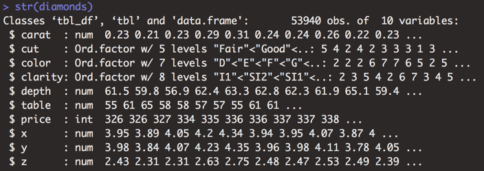
Figure 3.25: Data structure of the diamonds dataset.
3.3.10.3 Exercises
- Execute
str(mtcars) - Execute
str(diamonds) - Execute
str(npk) - Execute another built-in dataset or two. You can find a list of built-in datasets by executing
data()
3.3.11 Factors
A factor is another variable structure. Factors categorize character string values for a given variable. To determine whether your variable should be a factor, ask: Do the values in this variable belong in categories?
Example
If I have an experiment with a variable called Injection, my values might include:
DrugControl
Thus, Drug and Control are two different categorical values that the Injection variable can have.
Since
Injectionis categorical, it is referred to as a factor variable.Factor variables are useful for when you want to group a certain category for further analysis. The examples below suggest things you might want to know about your data:
I want to see what all of the subjects that are in the Drug group look like
I want to see what all of the subjects that are only in the
Controlgroup look likeI want to compare the categories of
Drugvs.Control
Let’s create another factor variable: Subject. Each value in Subject represents a subject ID – that is, 1 represents Subject #1 and 2 represents Subject #2. Even though the values in Subject appear to be numeric, they are not: Subject 1 is not less than Subject 2 and you cannot perform arithmetic on these values. Each subject is a category, where Subject #1’s data is separate from Subject #2’s data, etc. Injection is also a categorical variable. Rating is a numerical value, where a rating of 5 has some intrinsic value (there is a rank order where a rating of 5 is ranked differently from a rating of 3).
| Subject | Injection | Rating |
|---|---|---|
| 1 | Drug | 5 |
| 2 | Drug | 3 |
| 3 | Drug | 2 |
| 1 | Control | 9 |
| 2 | Control | 10 |
| 3 | Control | 8 |
The same thing applies below: Each value in the Subject variable is still a category. The Date variable contains date values as the numbers indicate some chronological order, rather than some numerical value. The Short Answer variable contains simple character values, where none of the values form a category as it currently stands. If the values, such as “It’s been a slow day”, were a category that everybody could select as an answer, then Short Answer would be a categorical variable.
| Subject | Date | Short Answer |
|---|---|---|
| Sam | 2019-02-05 | “It’s been a slow day” |
| Anna | 2019-01-07 | “Pretty standard day” |
| Michael | 2019-03-01 | “I’ve been pretty stressed” |
3.3.11.1 Exercises
Are the following variables factors/categorical? (yes/no)
Height measurement in cm
Age category (0-18, 19-25, 26-35, 36-60, 61+)
Age in years
Hair color (blonde, brunette, black, grey, other)
Exercise frequency (Sometimes, Never, Always)
Number of exercise hours per week
Subject name
Personality question asking whether you fit the description (true/false)
Year (1999, 2000, 2001…)
If the variable in the previous question was not a factor, what structure was it?