8 Internal validity in observational studies
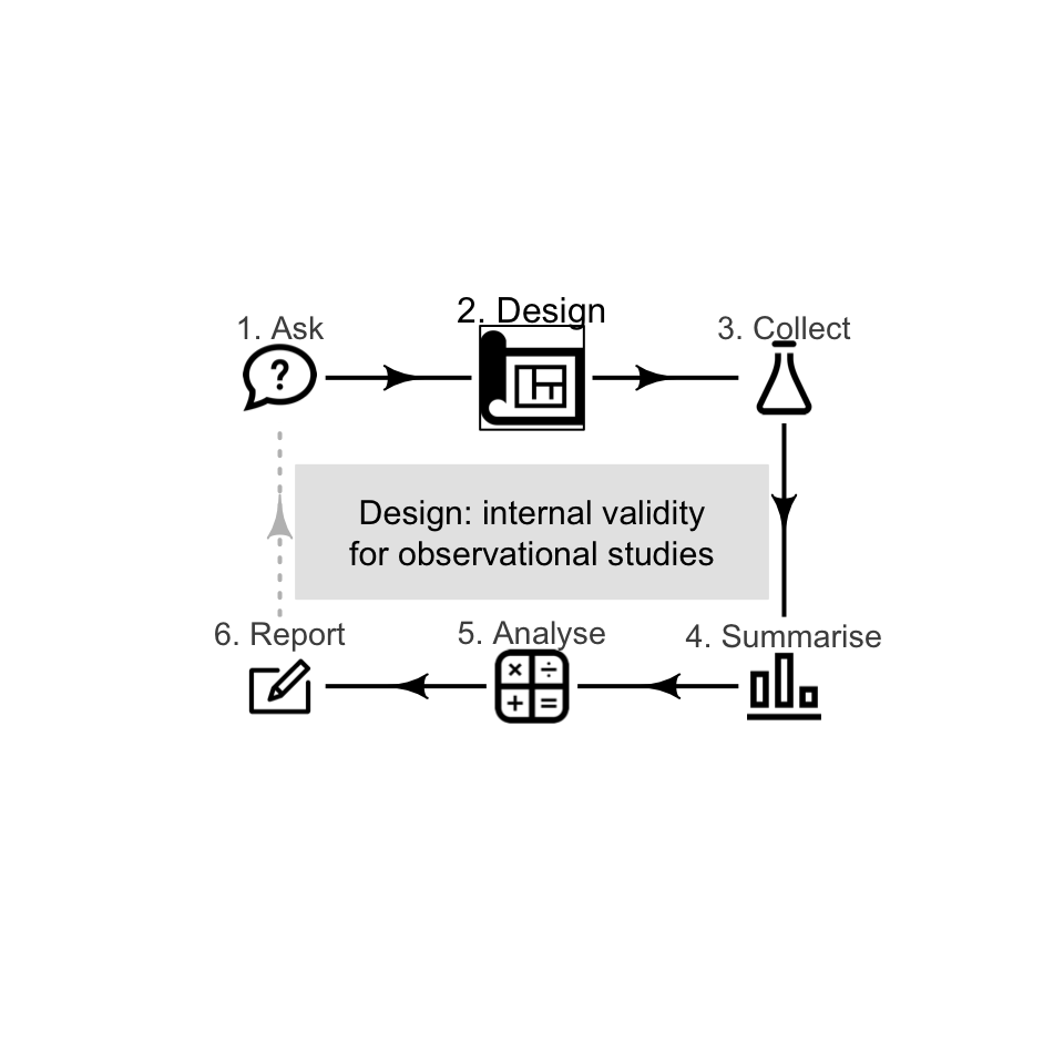
So far, you have learnt to ask a RQ and design experimental studies. In this chapter, you will learn about internal validity for observational studies. You will learn to:
- maximise the internal validity in observational studies.
- manage confounding in observational studies.
- explain, identify and manage the Hawthorne effect, the observer effect, the placebo effect and the carry-over effect in observational studies.
8.1 Introduction
In experimental studies, many aspects of the research design typically can be controlled by the researcher. In contrast, observational studies have fewer design features that can be controlled by the researchers. For example, random allocation of treatments is impossible since treatments are not imposed in observational studies, and hence confounding is a potential threat to internal validity in observational studies.
A well-designed study is needed to draw solid conclusions (Def. 6.2): a study with high internal validity (Sect. 6.1) and high external validity (Sect. 5.1)).
Specific design strategies for maximising internally validity are:
- Managing confounding (Sect. 8.2).
- Managing the Hawthorne effect (Sect. 8.3).
- Managing the observer effect (Sect. 8.4).
- Managing the carry-over effect (Sect. 8.5).
Since the placebo effect is concerned with individuals response to allocated treatments, it is not directly relevant to observational studies. Not all of these strategies are relevant to every study.
8.2 Managing confounding
In Sect. 7.2, methods were listed for managing confounding in experimental studies. Confounding can be managed for observational studies too:
- Restricting the study to a certain group. For example, Doll and Hill (1954) studied smoking in males aged under \(35\) years since, at the time of the study, 'lung cancer [was] relatively uncommon in women and rare in men under \(35\)' (p. 1452). The reason for the restriction should be justified if possible (as in this quotation).
- Blocking. Individuals that are similar to one another can be placed into different groups. Doll and Hill (1954), for example, could have found numerous pairs of smokers and non-smokers, with both subjects in each pair matched by having similar ages and alcohol-consumption habits.
- Analysing using special methods, after recording the values of potential confounding variables. Most studies involving people record the participants' age and sex, as these two variables are common confounders. Once a sample is obtained, recording this extra information usually requires little extra effort.
Randomly allocating individuals to groups is not possible in observational studies. For this reason, confounding is often a major threat to internal validity in observational studies, as individuals who are in one group may be different, in general, to those who are in another group.
Usually the best approach for observational studies is to record the values of any potential confounding variables, and use special analysis methods to understand the data. The groups being compared should be as similar as possible, apart from what is being studied. Hence, researchers often compare the comparison groups on potential confounding variables.
Record all extraneous variables likely to be important for understanding the individuals This may include information about the individuals in the study, and the circumstances of the individuals in the study.
Example 8.1 (Confounding) Froud, Beresford, and Cogger (2018) studied \(2599\) kiwifruit orchards, exploring the relationship between the time since a bacterial canker was first detected (in weeks), and the orchard productivity (in tray equivalents per hectare). The researchers also recorded extraneous variables such as 'whether or not the farm was organic', 'elevation of the orchard' and 'whether or not general fungicides were used'. These variables were used in their analysis to manage the potential effects of confounding.
Example 8.2 (Comparing study groups) An observational study compared the iron levels of active and sedentary women aged \(18\) to \(35\) (Woolf et al. 2009). The active (\(n = 28\)) and sedentary women (\(n = 28\)) were compared on a variety of characteristics (Table 8.1). The active women were similar to the sedentary women on these characteristics, but were (in general) slightly younger, slightly heavier, and slightly more likely to use hormonal contraceptives.
| Characteristic | Active women | Sedentary women |
|---|---|---|
| Average age (in years) | \(20\) | \(24\) |
| Average weight (in kg) | \(68\) | \(62\) |
| Percentage using hormonal contraceptives | \(13\) | \(11\) |
Observational studies can (and often do) have control groups (see Example 8.3). Indeed, one specific type of observational study is called a case-control study. However, individuals are not allocated to the control group by the researchers in observational studies, so the control and study groups may be very different, which may explain any differences in the outcome.
A study (Gunnarsson et al. 2017) examined the difference between two types of helicopter transfer (physician-staffed; non-physician-staffed) of patients with a specific type of myocardial infarction (STEMI). The purpose of the study was:
...to evaluate the characteristics and outcomes of physician-staffed HEMS (Physician-HEMS) versus non-physician-staffed (Standard-HEMS) in patients with STEMI.
--- Gunnarsson et al. (2017), p. 1
The researchers
...studied \(398\) STEMI patients transferred by either Physician-HEMS (\(n = 327\)) or Standard-HEMS (\(n = 71\)) for [...] intervention at \(2\) hospitals between 2006 and 2014.
--- Gunnarsson et al. (2017), p. 1
Since the study is an observational study (patients were not allocated by the researchers to the type of helicopter transport), the researchers recorded information about the patients being transported. They compared the patients in both groups, and found (for example) that both groups had similar average ages, and similar percentages of females and smokers, and so on. They also compared information about the transportation, and found (for example) that both groups had similar average flight times and flight distances.
One conclusion from the study was that 'Patients with STEMI transported by Standard-HEMS had longer transport times' (p. 1), but one limitation of the study was that:
The patient cohorts received treatment by \(2\) different care teams at two hospitals, which is a potential confounder despite similar baseline characteristics
--- Gunnarsson et al. (2017), p. 5
In other words, the difference between hospitals and the staff may have been a confounding variable.
Example 8.3 (Confounding) Doll and Hill (1950) studied smoking using a backward-direction study. The control group (those without lung cancer) was chosen to include very similar individuals to those in the lung-cancer group, in terms of age and sex. (That is, the numbers of females and males within each age group was very similar for those with and without lung cancer.)
8.3 Hawthorne effect and blinding individuals

In observational studies, individuals may or may not know they are being observed. For example, in an observational study where subjects' blood pressure is measured, subjects clearly know they are being observed, which has the potential to alter the subjects behaviour (for example, people become tense, called 'white-coat hypertension'; Pickering, Gerin, and Schwartz (2002)). As with experimental studies, efforts should be made to ensure that individuals do not know that they are being observed (the participants are blinded).
Example 8.4 (Hawthorne effect) A study (Wu et al. 2018) examined hand hygiene (HH) of staff in a tertiary teaching hospital, using covert observers (observers not obviously watching the HH practices) and overt observers (observers obviously about watching the HH practices). HH compliance was higher with overt observation (\(78\)%) than with covert observation (\(55\)%).
8.4 Observer effect and blinding researchers

The observer effect can impact observational as well as experimental studies. For example, consider a study measuring the blood pressure of smokers and non-smokers (Verdecchia et al. 1995). This study is observational (individuals cannot be allocated to be a smoker or non-smoker), but if the researchers know if an individual is a smoker when they measure blood pressure, then the observer effect could still impact the results (recalling that the observer effect is an unconscious effect). For example, the researchers may expect smokers to have a high blood pressure.
The observer effect could be managed by first measuring the blood pressure, and then asking if the individual was a smoker or not. That is, the researchers may be blinded to whether or not the subject is a smoker when they measure blood pressure. This may only be partially successful; the researcher may see the subject carrying cigarettes, or can smell smoke on their breath, for example. Nonetheless, since it may prove at least partially successful and is easy to implement, this strategy should form part of the research design.
Example 8.5 (Observer effect) Zimova et al. (2020) took photos of snowshoe hares, at various stages of moulting and in various environmental conditions. Eighteen independent observers were asked to rate the moult stage from the photographs (p. 4):
... images were randomly named and sorted, with the dates [...] removed to minimize observer expectancy bias [i.e., the observer effect].
A study of the scats of gray wolves was used to study their diet (Spaulding, Krausman, and Ballard 2000). A scat analysis is where humans examine the scat of carnivores to determine the prey. However, the accuracy of the results was questioned, due to 'perpetuation of the assumption that wolf scats contain only \(1\) prey item/scat' (p. 949).
The observers might be seeing what they expect to see: that "wolf scats contain only \(1\) prey item/scat".
8.5 Carry-over effect and washout periods

The carry-over effect is a possible compromise to internal validity in observational studies involving a within-individuals comparison. However, since treatments are not allocated in observational studies, carry-over effects may be difficult to prevent as washouts cannot be imposed, and the order of the conditions cannot be imposed. However, observing individuals exposed to Condition A then Condition B, and other individuals exposed to Condition B then Condition A, may be possible.
Example 8.6 (Carry-over effects) Norris (2005) studied the carry-over effect in ecological observational studies of animals (p. 181):
...individuals occupying poor quality winter habitat may experience reduced reproductive success the following breeding season when compared to individuals occupying high quality winter habitat.
8.6 Comments on blinding
Many comments about blinding made for experimental studies (Sect. 7.8) apply for observational studies also. In observational studies, blinding individuals may be (but is not always) easier than in experimental studies (Sect. 8.3). Blinding the researchers may be difficult, since the researchers need to record the value of the explanatory variable. One strategy (also see Sect. 7.5) is for one researcher can record the value of the response variable, and another can record the value of the explanatory variable.
Example 8.7 (Blinding in observational studies) Emerson et al. (2010) studied Achilles tendinopathy in gymnasts, by comparing \(40\) elite gymnasts with \(41\) controls of similar non-gymnasts. The authors state (p. 38):
Although the primary investigator was blind to the clinical status of the subjects, there was no blinding to whether each subject was in the gymnast or control group during image collection [...] However the examiner was blinded to both the clinical state and group of each subject when the images were reviewed.
The paper clearly explains who was blinded and to what parts of the study they were blinded.
8.7 Recording extraneous variables
Recording the values of possible extraneous variables is very important for observational studies, as it one of the few effective ways to manage confounding. The reasons for recording the values of extraneous variables, in Sect. 7.9, still apply:
To evaluate external validity by allowing the sample and population to be compared, to determine if the sample is representative of the population (Sect. 5.10).
-
To improve internal validity, by helping to manage confounding:
Example 8.8 (Poor internal validity) In the 1800s, Semmelweis recorded mortality rates of women after childbirth over many years (P. M. Dunn 2005) at two clinics:
- In Clinic 1, with male doctors delivering babies: \(9.9\)%.
- In Clinic 2, with female midwives delivering babies: \(3.4\)%.
Was the difference in mortality rate (the outcome) due to the sex of the person delivering the babies (the comparison)?
One possible confounder was the clinic; however, the clinic was eliminated as an explanation. For example, Clinic 2 was actually more overcrowded than Clinic 1, and the climate was similar for both clinics.
However, an important lurking variable was present. In the 1800s, the benefits of hand washing were not understood, nor commonplace. Many (male) doctors performed autopsies before delivering babies, without washing their hands between procedures. In contrast, autopsies were not performed by the (female) nurses.
The lurking variable was 'whether the baby was delivered by someone with clean hands', which was related to the mortality rate and to the sex of the person delivering the baby. The female midwives had clean hands, and hence the mortality rate was (relatively) low. The male doctors did not have clean hands, and hence the mortality rate was high.
After instituting hand washing for doctors, the mortality rate in Clinic 1 reduced to a rate similar to that in Clinic 2.
8.8 Chapter summary
Designing effective observational studies (Fig. 8.1) requires researchers to maximise internal validity. This can be achieved by managing confounding where possible, as confounding is often a major threat to the internal validity of observational studies. Confounding can be managed by restricting the study to certain groups; blocking; and/or through special analysis methods.
Random allocation is not possible in observational studies. For this reason, observing, measuring, assessing or recording all the information that is likely to be important for understanding the data is important, usually to be used in analysis. Well-designed observational studies also try to manage the carry-over effect, the Hawthorne effect, and the observer effect The placebo effect is not relevant.
Strategies for controlling these impacts are often not under the control of the researchers in observational studies. Recording the values of possible extraneous variables is very important for observational studies.
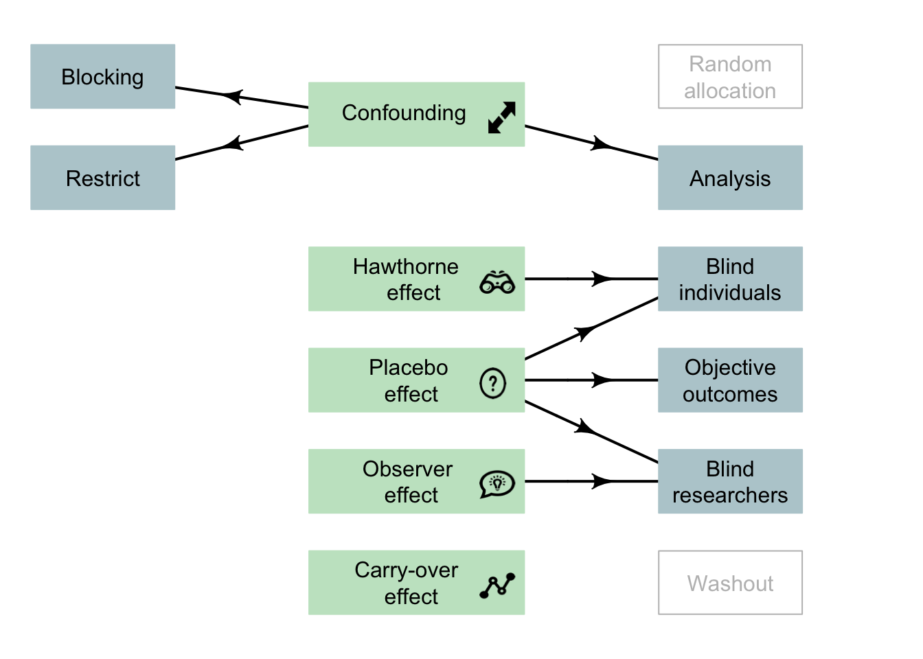
FIGURE 8.1: Design strategies for observational studies. Note: lurking variables become confounding variables when recorded in the study, and then they can be managed. The arrows indicate the main design strategy to (perhaps partially) manage the indicated potential bias. Not all strategies are possible for every study.
8.9 Quick review questions
Formwork is used in construction with reinforced concrete, and can be labour intensive. Mine et al. (2015) examined the relationship between the floor area of the building (in m2 per storey) and the number of hours of labour needed for constructing the formwork (in person-minutes per storey). The researchers also recorded the average age of the workers (in years); the average years of experience of the workers (in years); and the storey height (in meters) for each of \(n = 15\) multi-storey buildings in the study.
Two observers recorded the labour time by observing workers from the start to the end of the work.
- What is the explanatory variable?
- What is the response variable?
- What type of description is appropriate for the variable 'Average age of the workers'?
- What is the most likely way to manage confounding in this study?
- True or false: The carry-over effect is likely to be a big problem in this study.
- True or false: The Hawthorne effect is likely to be a big problem in this study.
- True or false: The placebo effect is likely to be a big problem in this study.
- True or false: Observer bias is likely to be a big problem in this study.
8.10 Exercises
Answers to odd-numbered exercises are available in App. E.
Exercise 8.1 Which of the following statements are true?
- Observational studies cannot have a control group.
- Only experimental studies can use random allocation to avoid confounding
- Only observational studies can manage the observer effect
- Only experimental studies can use random sampling
Exercise 8.2
A study compared the average amount of pollen returned to the hive per bee, for two types of native Australian bees: yellow and black carpenter bees, and green carpenter bees. In the study, the researchers also recorded the size of the hive, among other things. Why did they do this?Exercise 8.3 Consider this RQ (based on Teillet et al. (2010)): 'Among university students, is the taste of tap water different than the taste of bottled water?'
You want to answer this question using an observational study. Describe what these might look like for this study, and which are feasible: random allocation; blinding; double blinding; control; finding a random sample.
Exercise 8.4 Is the Hawthorne effect only a (potential) issue for experiments. Explain.
Exercise 8.5 A study of how well hospital patients sleep at night (Delaney et al. 2018) had the stated aim 'to investigate the perceived duration and quality of patient sleep'. In discussing the limitations of the study, the researchers state (p. 7):
The researchers made no attempt to deceive clinical staff regarding the nature of the study so the influence of the Hawthorne Effect should be considered. The presence of the observer and environmental monitoring equipment in the clinical environment could have altered behaviour among patients and nursing staff seeking to conform to the presumed research objectives. As a result, the findings reported may be an underestimation of the magnitude of the issues that affect sleep.
Discuss these limitations in terms of the language used in this chapter.
Exercise 8.6 Stafford, Daube, and Franklin (2010) studied smoking in alfresco restaurants in two cities in Western Australia. The concentration of particulate matter with a diameter smaller than or equal to \(2.5\) (per cubic metre of air) was recorded (PM2.5)from \(12\) cafes and \(16\) pubs. The researchers were interested in the relationship between PM2.5 and the number of smokers. They also recorded the wind strength (calm; light breeze; windy) and the amount of cover (fully open; overhead cover only; overhead cover and enclosed sides).
- What are the response and explanatory variables?
- What are the extraneous variables, if any?
Exercise 8.7 In a study of time spent applying sunscreen (Heerfordt et al. 2018), the Aim was to 'determine whether time spent on sunscreen application is related to the amount of sunscreen used' (p. 117). The study is described as follows (p. 118):
The volunteers were asked to apply the provided sunscreen [...] the way they would normally do on a sunny day at the beach in Denmark [...] The volunteers wore swimwear during the whole session. No other information was given. Participants applied sunscreen behind a curtain and were not observed during application. Measurements of time and sunscreen weight were made without the subjects' being aware of this.
- What are the response and explanatory variables?
- The researchers also recorded age, height, weight and body surface area of each participant. Why would they have done this?
- The researchers also compared the mean values of the response variable for males and females, and the mean values of the explanatory variable for males and females. Why would they have done this?
- What design features are evident in the quote?