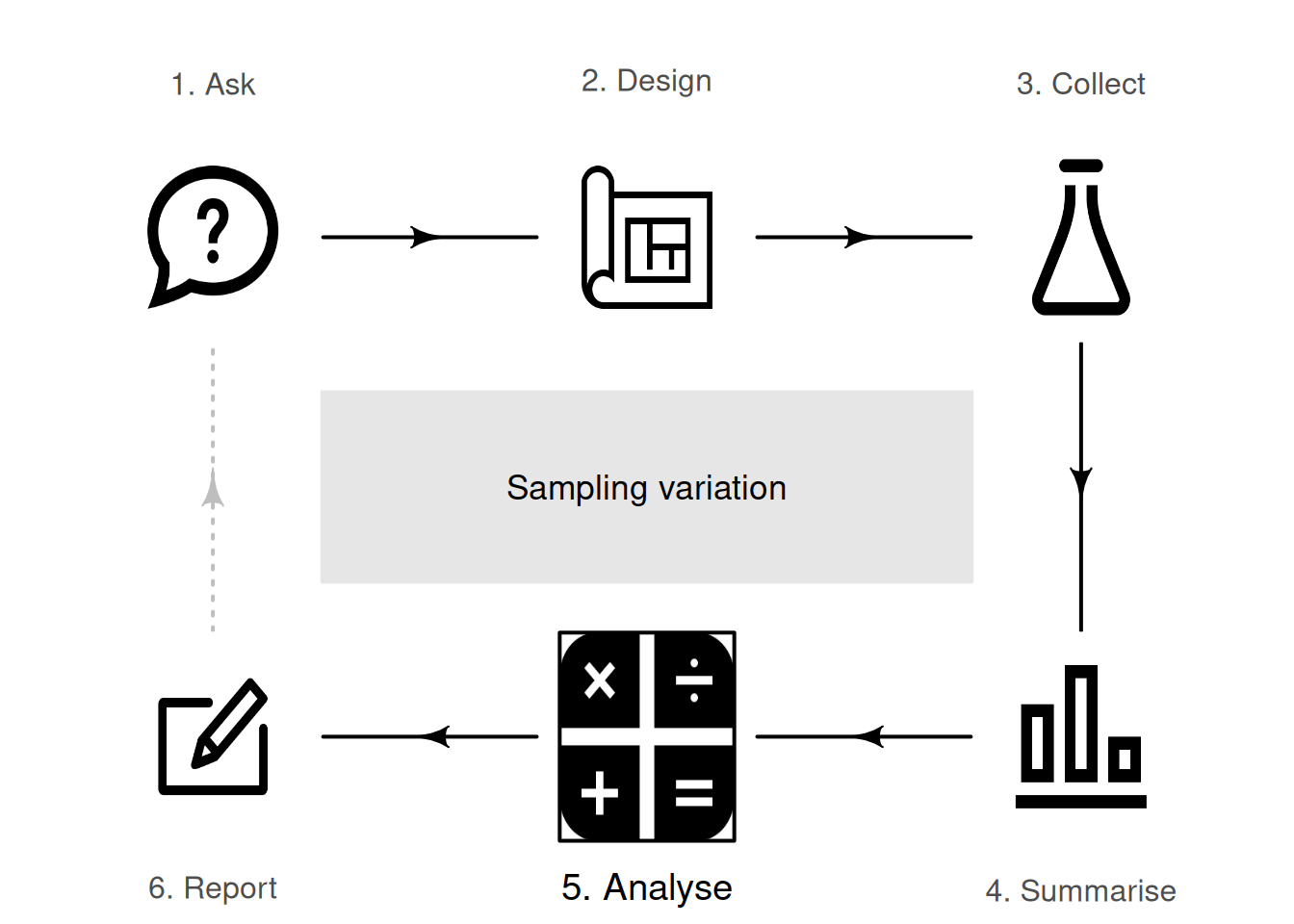
21 Sampling variation

So far, you have learnt to ask a RQ, design a study, describe and summarise the data, and understand the decision-making process. In this chapter, you will learn to:

explain what a sampling distribution describes.
explain the difference between variation between individuals and variation in sample statistics.
determine when a standard error is appropriate to use.
explain the difference between standard errors and standard deviations.

21.1 Introduction

The previous chapter introduced the decision-making process (Sect. 20.4) used in research:

Make an assumption about the population parameter.
Based on this assumption, describe what values the sample statistic might reasonably be expected from all possible samples.
Observe the sample data from just one of those may possible samples.
Decide if the sample statistic seems consistent with the expectation, or if it contradicts the expectation.

Realising that the sample studied is only one of countless possible samples that could have been chosen is important.

Remember: studying a sample leads to the following observations:

Every sample is likely to be different.
We observe just one of the many possible samples.
Every sample is likely to yield a different value for the sample statistic.
We observe just one of the many possible values for the statistic.

Since many values for the sample statistic are possible, the possible values of the sample statistic vary (called sampling variation) and have a distribution (called a sampling distribution).

Furthermore, under certain conditions, the variation of the sample statistic (such as the sample mean, etc.) from all possible samples can be described based on the assumption made about the parameter. As a result, the expected behaviour of these statistics can be described, so we know what to expect from the sample statistic when the assumption is true.

We saw this in Sect. 20.4: the sample proportion of red cards in a sample of $15$ varied from hand to hand, and was approximately distributed with a bell-shape. This bell-shaped distribution is formally called a normal distribution. This is no accident: Many sample statistics vary from sample to sample with an approximate normal distribution if certain conditions are met. We see examples of this in this chapter. Bell-shaped distributions are studied further in Chap. 22.

Any distribution that describes how a sample statistic varies for all possible samples is called a sampling distribution: how the value of the sample statistic varies from sample to sample for all possible samples. The sampling distribution often has a normal distribution shape.

Definition 21.1 (Sampling distribution) A sampling distribution is the distribution of some sample statistic, showing how its value varies from sample to sample.

21.2 Sample proportions have a distribution

Sample proportions, like all sample statistics, vary from sample to sample (Sect. 20.4); that is, sampling variation exists, so sample proportions have a sampling distribution.

Consider a European roulette wheel shown below in the animation: a ball is spun and can land on any number on the wheel from $0$ to $36$ (inclusive). Using the classical approach to probability, the probability of the ball landing on an odd number (an 'odd-spin') is $p = 18/37 = 0.486$. This is the population proportion.

If the wheel is spun (say) 15 times, the sample proportion of odd-spins in those 15 spins, denoted $\hat{p}$, will vary. But, how does $\hat{p}$ vary from one set of 15 spins to another set of 15 spins? Can we describe how the value of $\hat{p}$ varies?

Computer simulation can be used to demonstrate what happens if the wheel was spun, over and over again, for $n = 15$ spins each time, and the proportion of odd-spins was recorded for each repetition. The proportion of odd spins $\hat{p}$ can vary from sample to sample (sampling variation) for one sample of $n = 15$ spins, as shown by the histogram (Fig. 21.1, top left panel). The shape of the distribution is approximately bell shaped. We can see that, for many repetitions, $\hat{p}$ is rarely smaller than $0.2$, and rarely larger than $0.8$. That is, reasonable values to expect for $\hat{p}$ are between about $0.2$ and $0.8$.

If the wheel was spun (say) $n = 25$ times (rather than $15$ times), $\hat{p}$ again varies (Fig. 21.1, top right panel): the values of $\hat{p}$ vary from sample to sample. The same process can be repeated for many repetitions of (say) $n = 100$ and $n = 200$ spins (Fig. 21.1, bottom panels).

Notice that as the sample size $n$ gets larger, the distribution of the values of $\hat{p}$ look more like a bell-shaped (normal) distribution, and the variation gets smaller. With $200$ spins, for instance, observing a sample proportion smaller than $0.4$ or greater than $0.6$ seems highly unusual, but these are not uncommon at all for $15$ spins.

Example 21.1 (Reasonable values for $\hat{p}$) Suppose we spun a roulette wheel $100$ times, and observed $31$ even numbers. The sample proportion is $\hat{p} = 31/100 = 0.31$. From Fig. 21.1 (bottom left panel), a sample proportion this low almost never occurs in a sample of $100$ rolls.

We observed something that is very unlikely to occur. This suggests that we observed something highly unusual, or a problem exists with the wheel.

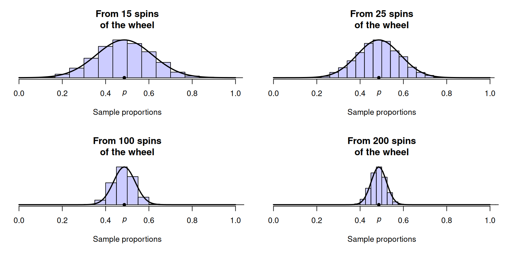
FIGURE 21.1: Sampling distributions for the proportion of roulette wheel spins that show an odd number, for set of rolls of varying sizes

The values of the sample proportion vary from sample to sample. The distribution of the possible values of the sample statistic (in this case the sample proportion) from sample to sample is called a sampling distribution.

Under certain conditions, the sampling distribution of a sample proportion is described by an approximate a normal distribution. In general, the approximation gets better as the sample size gets larger, and the possible values of $\hat{p}$ vary less as the sample size gets larger.

The mean of the sampling distribution is called the sampling mean; the standard deviation of the sampling distribution is called the standard error.

21.3 Sample means have a distribution

The sample mean, like all sample statistics, varies from sample to sample (Sect. 20.4); that is, sampling variation exists, so sample means have a sampling distribution.

Consider a European roulette wheel again (Sect. 21.2). Rather than recording the sample proportion of odd-spins, suppose the sample mean of the numbers spun was recorded. If the wheel is spun (say) $15$ times, the sample mean of the spins $\bar{x}$ will vary from one set of $15$ spins to another. How does it vary?

Again, computer simulation can be used to demonstrate what could happen if the wheel was spun $15$ times, over and over again, and the mean of the spun numbers was recorded for each repetition. Clearly, the sample mean spin $\bar{x}$ can vary from sample to sample (sampling variation) for $n = 15$ spins (Fig. 21.2, top left panel).

When $n = 15$, the sample mean $\bar{x}$ indeed varies from sample to sample. The shape of the distribution again is approximately bell shaped. If the wheel was spun more than $15$ times (say, $n = 50$ times) something similar occurs (Fig. 21.2, top right panel): the values of $\bar{x}$ vary from sample to sample, and the values have an approximate bell-shaped (normal) distribution. In fact, the values of $\bar{x}$ have a bell-shaped distribution for other numbers of spins also (Fig. 21.2, bottom panels).

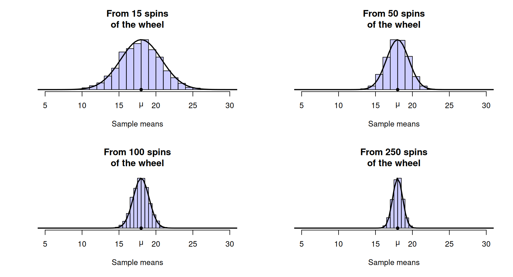
FIGURE 21.2: Sampling distributions for the mean of the numbers after a roulette wheel spins a certain number of times

The values of the sample mean vary from sample to sample. The distribution of the possible values of a sample statistic, in this case the sample mean, is called a sampling distribution.

Under certain conditions, the sampling distribution of a sample mean is described by an approximate a normal distribution. In general, the approximation gets better as the sample size gets larger, and the possible values of $\bar{x}$ vary less as the sample size gets larger.

The mean of the sampling distribution is called the sampling mean; the standard deviation of the sampling distribution is called the standard error (Fig. 21.3).

Example 21.2 (Reasonable values for $\bar{x}$) Suppose we spun a roulette wheel $100$ times, and the mean of the observed numbers was $\bar{x} = 18.9$. From Fig. 21.2 (bottom left panel), a sample mean with this value does not look unusual at all; it would occur reasonably frequently.

Nothing suggests that a problem exists with the wheel.

As we have seen, each sample is likely to be different, so any statistic is likely to be vary from sample to sample. (The value of the population parameter does not change.) This variation in the possible values of the observed sampling statistic is called sampling variation.

21.4 Sampling means and standard errors

As seen in the previous two sections, the value of a sample statistic varies from sample to sample. The statistic we observe depends on which one of the countless samples is selected, and hence which value of the sample statistic is observed.

This means that the possible values of sample statistics that we could potentially observe have a distribution (specifically, a sampling distribution); see Fig. 21.3. Perhaps surprisingly, under certain conditions, the sampling distribution is often a normal distribution, as we have seen.

The mean of this sampling distribution is called the sampling mean. The sampling mean is the average value of the sample statistic, across all possible samples.

Definition 21.2 (Sampling mean) The sampling mean is the mean of the sampling distribution of a statistic.

The standard deviation of this sampling distribution is called the standard error. The standard error measures the value of the sample statistic is likely to vary across, across all of the possible samples; see Fig. 21.3. The standard error is a measure of how precisely the sample statistic estimates the population parameter. If every possible sample (of a given size) was found, and the statistic computed from each sample, the standard deviation of all these estimates is the standard error.

Definition 21.3 (Standard error) A standard error is the standard deviation of the sampling distribution of a statistic.

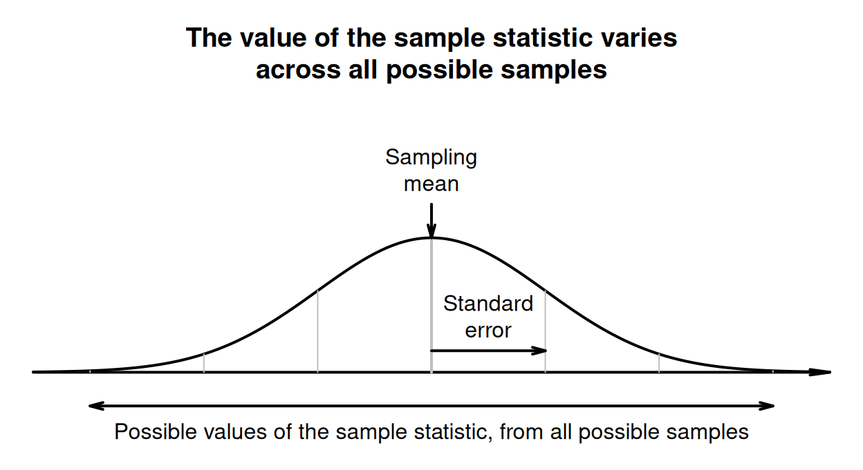
FIGURE 21.3: Describing how the value of the sample statistic varies across all possible samples

Figures 21.1 and 21.2 show that the variation in the values of the sample statistic get smaller for larger sample sizes. That is, the standard error gets smaller as the sample sizes get larger: the sample statistics show less variation for larger $n$.

This makes sense: larger samples generally produce more precise estimates. After all, that's the advantage of using larger samples: all else being equal, larger samples are preferred as they produce more precise estimates (Sect. 5.3).

Example 21.3 (Standard errors) In Fig. 21.2, a sample of $250$ (i.e., $250$ spins) is unlikely to produce a sample mean larger than $20$, or smaller than $15$. However, in a sample of size $15$ (i.e., $15$ spins) sample means near $15$ and $20$ are quite commonplace.

In samples of size $100$, the variation in the mean spin is smaller than in samples of size $15$. Hence, the standard error (the standard deviation of the sampling normal distributions) will be smaller for samples of size $250$ than for samples of size $15$.

For many sample statistics, the variation from sample to sample can be approximately described by a normal distribution (the sampling distribution) if certain conditions are met (Sect. 21.1). Furthermore, the standard deviation of this normal distribution is called the standard error. The standard error is a special name given to the standard deviation that describes the variation in a sample estimate that varies from sample to sample.

The standard error is an unfortunate term: it is not an error, or even standard. (For example, there is no such thing as a 'non-standard error'.)

21.5 Standard deviation vs standard error

Even experienced researchers confuse the meaning and the usage of the terms standard deviation and standard error (Ko et al. 2014). Understanding the difference is important.

The standard deviation, in general, quantifies the amount of variation in any quantity that varies. The standard error specifically refers to the standard deviation that describes a sampling distribution.

Typically, standard deviations describe the variation in the individuals in a sample: how observations vary from individual to individual. The standard error is only used to describe how sample estimates vary from sample to sample (i.e., to describe the precision of sample estimates).

The standard error is a standard deviation, but is only used to describe the variation in sampling distributions. Any numerical quantity estimated from a sample (a statistic) can vary from sample to sample, and so has sampling variation, a sampling distribution, and hence a standard error. (Not all sampling distributions are normal distributions, however.)

Any quantity estimated from a sample (a statistic) has a standard error.

The standard error is often abbreviated to 'SE' or 's.e.'. For example, the 'standard error of the sample mean' is often written $\text{s.e.}(\bar{x})$, and the 'standard error of the sample proportion' is often written $\text{s.e.}(\hat{p})$.

21.6 Chapter summary

A sampling distribution describes how all possible values of a sample statistic vary from sample to sample. Under certain circumstances, the sampling distribution often can be described by a normal distribution. The standard deviation of this normal distribution is called a standard error. The standard error is the name specifically given to the standard deviation that describes the variation in the sample statistic across all possible samples.

21.7 Quick review questions

Why is phrase 'the standard error of the population proportion' inappropriate?
Because only sample statistics have values that vary from sample to sample.Because proportions do not have a standard error.Because proportions only have a standard deviation.Because proportions come from qualitative data.
Which one the following does not have a standard error?
The sample mean.The difference between two sample means.The sample proportion.The sample odds ratio.The sample size.
True or false: Sampling variation refers to how sample sizes vary.
True or false: Sampling distributions describe parameters.
True or false: Statistics do not vary from sample to sample.
True or false: Populations are numerically summarised using parameters
True of false: The standard deviation is a standard error of something quite specific.
True or false: Sampling distributions are always normal distributions.
True or false: Sampling variation measures the amount of variation in the individuals in the sample (for the variable of interest).
True or false: The standard error measures the size of the error when we use a sample to estimate a population.
True or false: In general, a standard deviation measures the amount of variation.
True or false: The standard error is a standard deviation with a specific use.
True or false: Sampling variation measures the size of the sample.

21.8 Exercises

Answers to odd-numbered exercises are available in App. E.

Exercise 21.1 In the following scenarios, would a standard deviation or a standard error be the appropriate way to measure the amount of variation? Explain.

Researchers are studying the spending habits of customers. They would like to measure the variation in the amount spent by shoppers per transaction at a supermarket.
Researchers are studying the time it takes for inner-city office workers to travel to work each morning. They would like to determine the precision with which their estimate (a mean of $47$ mins) has been measured.
A study examined the effect of taking a pain-relieving drug on children. The researchers wish to describe the sample they used in the study, including a description of how the ages of the children in the study vary.
A study examined the effect of taking a pain-relieving drug in teenagers. The researchers wished to report the percentage of teenagers in the sample that experienced side-effects with some indication of the precision of that estimate.

Exercise 21.2 Which of the following have a standard error?

The population proportion.
The sample median.
The sample IQR.

The sample standard deviation.
The population odds.

Exercise 21.3 A research article (Nagele 2003) made this statement:

... authors often [incorrectly] use the standard error of the mean (SEM) to describe the variability of their sample...

What is wrong with using the standard error of the mean to describe the sample? How would you explain the difference between the standard error and the standard deviation to researchers who misuse the terms?

20 Making decisions

22 Distributions and models