28 More details about hypothesis testing

You have learnt to ask an RQ, design a study, classify and summarise the data, construct confidence intervals, and conduct hypothesis tests. In this chapter, you will learn more about hypothesis tests. You will learn to:

understand the process of hypothesis testing.
communicate the results of hypothesis tests.
interpret $P$ -values.

28.1 Introduction

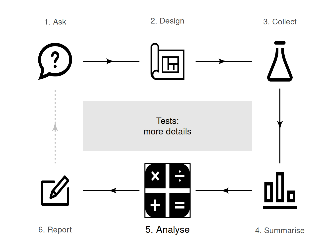
In Chaps. 26 and 27, hypothesis tests for one proportion and one mean were studied. Later chapters discuss hypothesis tests in other contexts, too. However, the general approach to hypothesis testing is the same for any hypothesis test. This chapter discusses some general ideas in hypothesis testing:

the assumptions and forming hypotheses (Sect. 28.2).
the expectations of the statistic, as described by the sampling distribution (Sect. 28.3).
the observations and the test statistic (Sect. 28.4).
quantifying the consistency between the values of the statistic and parameter using $P$ -values (Sect. 28.5).
interpreting $P$ -values (Sect. 28.6).
how conclusions can go wrong (Sect. 28.7).
wording conclusions (Sect. 28.8).
practical importance and statistical significance (Sect. 28.9).
statistical validity in hypothesis testing (Sect. 28.10).

28.2 More details about hypotheses and assumptions

Two statistical hypotheses are stated about the population parameter: the null hypothesis $H_0$ , and the alternative hypothesis $H_1$ . The null hypothesis is assumed to be true, and retained unless persuasive evidence exists to change our mind.

The word hypothesis means 'a possible explanation'.

Scientific hypotheses refer to potential scientific explanations that can be tested by collecting data. For example, an engineer may hypothesise that replacing sand with glass in the manufacture of concrete will produce desirable characteristics (Devaraj et al. 2021). Scientific hypotheses lead to research questions.

Statistical hypotheses refer to statements made about a parameter that may explain the value of a sample statistic. The statistical hypotheses are the foundation of the logic of hypothesis testing. One of the statistical hypotheses usually align with the scientific hypothesis.

This book discusses forming statistical hypotheses.

28.2.1 Null hypotheses

Statistical hypotheses are always about a parameter. Hypothesising, for example, that the sample mean body temperature (in Chap. 27) is equal to $37.0$ ^oC is silly: the sample mean clearly is $36.8052$ ^oC for the sample taken, and its value will vary from sample to sample anyway. The RQ is about the unknown population: the P in POCI stands for Population.

The null hypothesis $H_0$ proposes that sampling variation is why the value of the statistic (such as the sample mean) is not the same as the assumed value of the parameter (such as the population mean). Every sample is different, and the observed data is from just one of the many possible samples. The value of the statistic will vary from sample to sample; the statistic may not be equal to the parameter, just because of the random sample obtained and sampling variation.

Definition 28.1 (Null hypothesis) The null hypothesis proposes that sampling variation explains the discrepancy between the proposed value of the parameter, and the observed value of the statistic.

Null hypotheses always contain an 'equals', because (as part of the decision-making process) a specific value must be assumed for the parameter, so we can describe what we might expect from the sample. For example: the population mean equals $100$ , is less than or equal to $100$ ( $\mu\le100$ ), or is more than or equal to $100$ ( $\mu\ge100$ ).

The null hypothesis always assumes the discrepancy between the statistic and the assumed value of the parameter is due to sampling variation. This may mean, for example:

there is no change in the value of the parameter compared to an established or accepted value (for descriptive RQs), such as in the body-temperature example in Chap. 27.
there is no change in the value of the parameter for the units of analysis (i.e., for repeated-measures RQs).
there is no difference between the value of the parameter in two (or more) groups (i.e., for relational RQs).
there is no relationship between the variables, as measured by some parameter (for correlational RQs).

The null hypothesis always has the form 'no difference, no change, no relationship' regarding the population parameter. It is the 'sampling variation' explanation for the discrepancy between the value of the parameter and the value of the statistic.

Defining the parameter carefully is important!

28.2.2 Alternative hypotheses

The alternative hypothesis $H_1$ (or $H_a$ ) offers another possible reason why the value of the statistic (such as the sample proportion) is not the same as the proposed value of the parameter (such as the population proportion): the value of the parameter really is not the value claimed in the null hypothesis.

Definition 28.2 (Alternative hypothesis) The alternative hypothesis proposes that the discrepancy between the proposed value of the parameter and the observed value of the statistic cannot be explained by sampling variation. It proposes that the value of the parameter is not the value claimed in the null hypothesis.

Alternative hypotheses can be one-tailed or two-tailed. A two-tailed alternative hypothesis means, for example, that the population mean could be either smaller or larger than what is claimed. A one-tailed alternative hypothesis admits only one of those two possibilities. Most (but certainly not all) hypothesis tests are two-tailed.

The decision about whether the alternative hypothesis is one- or two-tailed depends on what the RQ asks (not by looking at the data). The RQ and hypotheses should (in principle) be formed before the data are obtained, or at least before looking at the data if the data are already collected.

The idea of hypothesis testing is the same whether the alternative hypothesis is one- or two-tailed: based on the data and the statistic, a decision is to be made about whether the data provides persuasive evidence to support the alternative hypothesis.

Example 28.1 (Alternative hypotheses) For the body-temperature study (Chap. 27), the alternative hypothesis is two-tailed (i.e., $H_1$ : $\mu \ne 37.0$ ): the RQ asks if the population mean is $37.0$ ^oC or not. Two possibilities are considered: that $\mu$ could be either larger or smaller than $37.0$ .

A one-tailed alternative hypothesis would be appropriate if the RQ asked 'Is the population mean internal body temperature greater than $37.0$ ^oC?' (i.e., $H_1$ : $\mu > 37.0$ ), or 'Is the population mean internal body temperature smaller than $37.0$ ^oC?' (i.e., $H_1$ : $\mu < 37.0$ ). One-tailed RQs such as these would only be asked if there were good scientific reasons to suspect a difference in one direction specifically.

Important points about forming hypotheses:

hypotheses always concern a population parameter.
hypotheses emerge from the RQ (not the data).
null hypothesis always have the form 'no difference, no change, no relationship' (i.e., sampling variation explains the discrepancy between the values of the parameter and statistic).
null hypotheses always contain an 'equals'.
alternative hypotheses may be one- or two-tailed, depending on the RQ.

28.3 More details about sampling distributions and expectations

The sampling distribution describes, approximately, how the value of the statistic (such as $\hat{p}$ or $\bar{x}$ ) varies across all possible samples, when $H_0$ is true; it describes the sampling distribution. Some sampling distributions have an approximate normal distribution.

When the sampling distribution is described by a normal distribution, the mean of the normal distribution (the sampling mean) is the parameter value given in the assumption ( $H_0$ ), and the standard deviation of the normal distribution is called the standard error. However, not all sampling distributions are normal distributions.

The variation in the sampling distribution (as measured by the standard error) depends on the sample size. For example, suppose $p$ is defined as the probability of rolling a ⚀ on a die. In one roll, finding a sample proportion of $\hat{p} = 1$ , is not unreasonable. However, in $20\,000$ rolls, a sample proportion of $\hat{p} = 1$ would be incredibly unlikely for a fair die.

28.4 More details about observations and the test statistic

The sampling distribution describes what values the statistic can take over all possible samples of a given size. When the sampling distribution has an approximate normal distribution, the observed value of the test statistic is $\text{test statistic} = \frac{\text{value of sample statistic} - \text{centre of the sampling distribution}} {\text{standard deviation of the sampling distribution}}.$ The 'standard deviation of the sampling distribution' is called the standard error of the statistic. This is called a 'test statistic', since the calculation is based on sample data (so it is a statistic) and used in a hypothesis test. This test statistic may be a $z$ -score or a $t$ -score. Other test statistics, when the sampling distribution is not described by a normal distribution, are used too (as in Chap. 31).

A $t$ -score and $z$ -score both measure the number of standard deviations that a value is from the mean: $\frac{\text{a value that varies} - \text{mean of the distribution}} {\text{standard deviation of the distribution}}.$ Then:

if the quantity that varies is an individual observation $x$ , the measure of variation is the standard deviation of the individual observations.
if the quantity that varies is a sample statistic, the measure of variation is a standard error, which measures the variation in a sample statistic.

When conducting hypothesis tests about means, the test statistic is a $t$ -score if the measure of variation uses a sample standard deviation.

28.5 More details about finding $P$ -values

When the sampling distribution has an approximate normal distribution, $P$ -values can be approximated (using the $68$ -- $95$ -- $99.7$ rule or tables), as demonstrated in Sect. 26.7. The $P$ -value is the area more extreme than the calculated $z$ - or $t$ -score (i.e., in the tails of the distribution). The $68$ -- $95$ -- $99.7$ rule can be used to approximate this tail area (when the sampling distribution has an approximate normal distribution).

A lower-case $p$ or upper-case $P$ can be used to denote a $P$ -value. We use an upper-case $P$ , since we use $p$ to denote a population proportion.

For two-tailed tests, the $P$ -value is the combined area in the left and right tails. For one-tailed tests, the $P$ -value is the area in just the left or right tail (as appropriate, according to the alternative hypothesis; see Sect. 27.9).

If the sampling distribution has an approximate normal distribution, the one-tailed $P$ -value is half the value of the two-tailed $P$ -value.

Some software always reports two-tailed $P$ -values.

More accurate approximations of the $P$ -value can be found using tables. Precise $P$ -values are found using the $P$ -values from software output.

28.6 More details about interpreting $P$ -values

Understanding $P$ -values requires care.

Definition 28.3 (P-value) A $P$ -value is the likelihood of observing the sample statistic (or something more extreme) over repeated sampling, under the assumption that the null hypothesis about the population parameter is true.

Since the null hypothesis is initially assumed true, the onus is on the data to present evidence to contradict the null hypothesis. That is, the null hypothesis is retained unless persuasive evidence suggests otherwise.

Conclusions are always about the parameters. $P$ -values tell us about the unknown parameters, based on the data from one of the many possible values of the statistic.

A 'big' $P$ -value means that the sample statistic (such as $\hat{p}$ ) could reasonably have occurred through sampling variation in one of the many possible samples, if the assumption made about the parameter (stated in $H_0$ ) was true. A 'small' $P$ -value means that the sample statistic (such as $\hat{p}$ ) is unlikely to have occurred through sampling variation in one of the many possible samples, if the assumption made about the parameter (stated in $H_0$ ) was true. 'Small' $P$ -values provide persuasive evidence to support the alternative hypothesis.

Commonly, a $P$ -value smaller than $5$ % (or $0.05$ ) is considered 'small' but this is arbitrary, and sometimes the threshold is discipline-dependent. More reasonably, $P$ -values should be interpreted as giving varying degrees of evidence in support of the alternative hypothesis (Table 28.1), but these too are only guidelines.

The threshold for a 'small' $P$ -value is very commonly $0.05$ , but this is arbitrary and not universal. There is nothing special about the value $0.05$ , and there is very little difference in the meaning of a $P$ -value of $0.051$ and a $P$ -value of $0.049$ .

TABLE 28.1: A guideline for interpreting $P$ -values. $P$ -values should be interpreted in context, and indicate the strength of evidence to support the alternative hypothesis.
If the $P$ -value is...	Write the conclusion as...
Larger than 0.10	Insufficient evidence to support $H_1$
Between 0.05 and 0.10	Slight evidence to support $H_1$
Between 0.01 and 0.05	Moderate evidence to support $H_1$
Between 0.001 and 0.01	Strong evidence to support $H_1$
Smaller than 0.001	Very strong evidence to support $H_1$

Identifying a $P$ -value of $0.05$ as 'small' (and hence providing 'persuasive evidence' to support $H_1$ ) is arbitrary; it means that, if $H_0$ is true, there is a $1$ -in- $20$ chance that the value of the statistic (or a value more extreme) would be observed due to sampling variation. In many situations, the evidence must be more persuasive than this.

To appreciate the concept of a $0.05$ (or a $1$ -in- $20$ ) chance:

the probability of throwing $5$ or more heads in a row using a fair coin is about $0.063$ .
the probability of drawing a black Ace from a pack of cards is about $0.038$ .
the probability of rolling two or more consecutive throws of a ⚅ is about $0.033$ .

These events are improbable, without being essentially impossible.

$P$ -values are commonly used in research, but must be used and interpreted correctly (Greenland et al. 2016). Specifically:

a $P$ -value is not the probability that the null hypothesis is true.
a $P$ -value does not prove anything (only one possible sample was studied).
a big $P$ -value does not mean the null hypothesis $H_0$ is true, or that $H_1$ is false.
a small $P$ -value does not mean the null hypothesis $H_0$ is false, or that $H_1$ is true.
a small $P$ -value does not mean the results are practically important (Sect. 28.9).
a small $P$ -value does not necessarily mean a large difference between the statistic and parameter; it means that the difference (whether large or small) could not reasonably be attributed to sampling variation (chance).

$P$ -values are never exactly zero. Some software reports very small $P$ -values as ' $P < 0.001$ ' (i.e., the $P$ -value is smaller than $0.001$ ). Some software reports very small $P$ -values as ' $P = 0.000$ ' (i.e., zero to three decimal places). In either case, we should still write $P < 0.001$ .

Some software only reports two-tailed $P$ -values.

Sometimes the results of a study are reported as being statistically significant. This usually means that the $P$ -value is less than $0.05$ , though a different $P$ -value is sometimes used as the 'threshold', so check!

To avoid confusion, the word 'significant' should be avoided in writing about research unless 'statistical significance' is actually meant. In other situations, consider using words like 'substantial'.

28.7 More details about how conclusions can go wrong

Hypothesis testing concerns making a decision about a population using sample information. Since the observed sample is just one of countless possible samples that could have been observed, making an incorrect conclusion is always a possibility.

Two mistakes can be made when making a conclusion:

incorrectly concluding that evidence supports the alternative hypothesis. Of course, the researchers do not know they are incorrect, but the possibility of making this mistake is always present. This is a false positive, or a Type I error.
incorrectly concluding there is no evidence to support the alternative hypothesis. Of course, the researchers do not know they are incorrect, but the possibility of making this mistake is always present. This is a false negative, or a Type II error.

Ideally, neither of these errors would be made; however, sampling variation means that neither can ever be completely eliminated. In practice, hypothesis testing begins by assuming the null hypothesis is true, and hence places the onus on the data to provide persuasive evidence in favour of the alternative hypothesis. This means researchers usually prioritise minimising the chance of a Type I error.

A Type I error is like declaring an innocent person guilty (recall: innocence is presumed in the judicial system). Similarly, a Type II error is like declaring a guilty person innocent. The law generally sees a Type I error as more grievous than a Type II error, just as in research. In general, larger sample sizes reduce the probability of making Type I and Type II errors.

In medical contexts, the terms sensitivity and specificity are often used rather than the terms Type I and Type II errors. Sensitivity is the probability of a positive test result among those with the disease, and specificity is the probability of a negative test result among those without the disease. High sensitivity is associated with a low chance of Type II error, and higher specificity is associated with a low chance of a Type I.

Example 28.2 (Type I errors) For the body-temperature example (Chap. 27), the conclusion was that the sample provided very strong evidence that the population mean body temperature was not $37.0$ ^oC. However, in truth, the mean internal body may not have changed, and is still $37.0$ ^oC; that is, the null hypothesis actually is true, but we incorrectly decided it was probably not true.

This would be a Type I error: we incorrectly concluded that the evidence supported the alternative hypothesis. Of course, since the value of $\mu$ is unknown, we do not know if we have made a Type I error or not.

28.8 More details about writing conclusions

In general, communicating the result of a hypothesis test requires stating:

the answer to the RQ.
the evidence used to reach that conclusion (such as the $t$ -score and $P$ -value, clarifying if the $P$ -value is one-tailed or two-tailed).
sample summary statistics (such as sample means, with CIs and sample sizes).

Since we initially assume the null hypothesis is true, conclusions are worded (in context) in terms of how strongly the evidence supports the alternative hypothesis.

Since the null hypothesis is initially assumed to be true, the onus is on the data to provide evidence in support of the alternative hypothesis: the null hypothesis is retained unless persuasive evidence suggests otherwise. Hence, conclusions are always worded in terms of how much evidence supports the alternative hypothesis.

We do not say whether the evidence supports the null hypothesis; the null hypothesis is already assumed to be true. Even if the current sample presents no evidence to contradict the assumption, future evidence may emerge. That is:

'No evidence of a difference' is not the same as 'evidence of no difference'.

Example 28.3 (No evidence of a difference) Suppose we test if the mean internal body temperature remains at $37.0$ ^oC (Chap. 27). Suppose we found no evidence that the internal body temperature had changed. This does not provide evidence that the mean internal body temperature is $37.0$ ^oC. It just means that the sample provided no evidence to change our initial assumption that the mean internal body temperature is $37.0$ ^oC.

28.9 More details about practical importance, statistical significance

Hypothesis tests assess statistical significance, which answers the question: 'Can sampling variation reasonably explain the discrepancy between the value of the statistic and the assumed value of the parameter?' Even very small discrepancies between the statistic and the parameter can be statistically different if the sample size is sufficiently large.

In contrast, practical importance answers the question: 'Is the discrepancy between the values of the statistic and the parameter of any importance in practice?' Whether a result is of practical importance depends upon the context: what the data are being used for. 'Practical importance' and 'statistical significance' are separate issues.

Example 28.4 (Practical importance) In the body-temperature study (Sect. 27.1), very strong evidence exists that the mean body temperature had changed ('statistical significance'). But the change was so small that, for most purposes, it has no practical importance. In other (e.g., medical) situations, it may have practical importance.

Example 28.5 (Practical importance) Maunder et al. (2020) studied the use of herbal medicines for weight loss, and found that the intervention (p. 891)

... resulted in a statistically significant weight loss compared to placebo, although this was not considered clinically significant.

This means that the difference in mean weight loss between the placebo and intervention groups was unlikely to be explained by chance ( $P < 0.001$ ; i.e., 'statistical significant'), but the difference was so small that it was unlikely to be of any use in practice ('practical importance'). In this context, the researchers decided that a weight loss of at least $2.5\,\text{kg}$ was of practical importance. However, in the study, the sample mean weight loss was $1.61\,\text{kg}$ .

28.10 More details about statistical validity

When performing hypothesis tests, statistical validity conditions must be true to ensure that the mathematics behind computing the $P$ -value is sound. For instance, the statistical validity conditions may ensure that the sampling distribution is sufficiently like a normal distribution for the $68$ -- $95$ -- $99.7$ rule to apply.

If the statistical validity conditions are not met, the $P$ -values (and hence conclusions) may be inappropriate or only approximately correct.

28.11 Chapter summary

Hypothesis testing formalises the decision-making process. Starting with an assumption about a parameter of interest, a description of what values the statistic might take is produced (the sampling distribution): this describes what values the statistic is expected to take over all possible samples. This sampling distribution is often a normal distribution.

The statistic (the sample estimate) is then observed, and a test statistic is computed to quantify the discrepancy between the values of the parameter (given in $H_0$ ) and statistic. Using a $P$ -value, a decision is made about whether the sample evidence supports or contradicts the initial assumption, and hence a conclusion is made. When the sampling distribution is an approximate normal distribution, the test statistic is a $t$ -score or $z$ -score, and $P$ -values can often be approximated using the $68$ -- $95$ -- $99.7$ rule.

28.12 Quick review questions

Are the following statements true or false?

When a $P$ -value is very small, a very large difference must exist between the statistic and parameter.
The alternative hypothesis is one-tailed if the sample statistic is larger than the hypothesised population mean.
When the sampling distribution has an approximate normal distribution, the standard deviation of this normal distribution is called the standard error.
Both $z$ -scores and $t$ -scores are test statistics.
$P$ -values can never be exactly zero.
A $P$ -value is the probability that the null hypothesis is true.

Select the correct answer:

What is wrong (if anything) with this null hypothesis: $H_0 = 37$ ?

0 of 7 correct

28.13 Exercises

Answers to odd-numbered exercises are given at the end of the book.

Exercise 28.1 Assuming the statistical validity conditions are satisfied, use the $68$ -- $95$ -- $99.7$ rule to approximate the two-tailed $P$ -value if:

the $t$ -score is $3.4$ .
the $t$ -score is $-2.9$ .

the $z$ -score is $-2.1$ .
the $t$ -score is $-6.7$ .

Exercise 28.2 Assuming the statistical validity conditions are satisfied, use the $68$ -- $95$ -- $99.7$ rule to approximate the two-tailed $P$ -value if:

the $z$ -score is $1.05$ .
the $t$ -score is $-1.3$ .

the $t$ -score is $6.7$ .
the $t$ -score is $0.1$ .

Exercise 28.3 Consider the test statistics in Exercise 28.1. Use the $68$ -- $95$ -- $99.7$ rule to approximate the one-tailed $P$ -values in each case.

Exercise 28.4 Consider the test statistics in Exercise 28.2. Use the $68$ -- $95$ -- $99.7$ rule to approximate the one-tailed $P$ -values in each case.

Exercise 28.5 Suppose a hypothesis test results in a $P$ -value of $0.0501$ . What would we conclude? What if the $P$ -value was $0.0499$ ? Comment.

Exercise 28.6 Suppose a hypothesis test results in a $P$ -value of $0.011$ . What would we conclude? What if the $P$ -value was $0.009$ ? Comment.

Exercise 28.7 Consider the study to determine if the mean body temperature (Chap. 27) was $37.0$ ^oC, where $\bar{x} = 36.8052$ ^oC. Explain why each of these sets of hypotheses are incorrect.

$H_0$ : $\bar{x} = 37.0$ ; $H_1$ : $\bar{x} \ne 37.0$ .
$H_0$ : $\mu = 37$ ; $H_1$ : $\mu > 37$ .
$H_0$ : $\mu = 37$ ; $H_1$ : $\mu = 36.8052$ .

$H_0$ : $\bar{x} = 36.8052$ ; $H_1$ : $\bar{x} > 36.8052$ .
$H_0$ : $\mu = 36.8052$ ; $H_1$ : $\mu \ne 36.8052$ .
$H_0$ : $\mu > 37.0$ ; $H_1$ : $\bar{x} > 37.0$ .

Exercise 28.8 Consider the study to determine if a die was loaded (Chap. 26) by studying the proportion of rolls that showed a ⚀, and where $\hat{p} = 0.41$ . Explain why each of these sets of hypotheses are incorrect.

$H_0$ : $\hat{p} = 1/6$ ; $H_1$ : $\hat{p} \ne 1/6$ .
$H_0$ : ${} = 1/6$ ; $H_1$ : ${} \ne 1/6$ .
$H_0$ : $p = 1/6$ ; $H_1$ : $\hat{p} = 0.41$ .

$H_0$ : $\hat{p} = 1/6$ ; $H_1$ : $\hat{p} = 0.41$ .
$H_0$ : $p = 1/6$ ; $H_1$ : $p > 1/6$ .
$H_0$ : $p = 1/6$ ; $H_1$ : $p = 0.41$ .

Exercise 28.9 The recommended daily energy intake for women is $7\,725$ kJ (for a particular cohort, in a particular country; Altman (1991)). The daily energy intake for $11$ women was measured to see if this is being adhered to. The RQ was 'Is the population mean daily energy intake $7\,725$ kJ?'

The test produced $P = 0.018$ . What, if anything, is wrong with these conclusions after completing the hypothesis test?

There is moderate evidence ( $P = 0.018$ ) that the energy intake is not meeting the recommended daily energy intake.
There is moderate evidence ( $P = 0.018$ ) that the sample mean energy intake is not meeting the recommended daily energy intake.
There is moderate evidence ( $P = 0.018$ ) that the population energy intake is not meeting the recommended daily energy intake.
The study proves that the population energy intake is not meeting the recommended daily energy intake ( $P = 0.018$ ).
There is some evidence that the population energy intake is not meeting the recommended daily energy intake ( $P < 0.018$ ).

Exercise 28.10 [Dataset: Battery] A study compared ALDI batteries to another brand of battery. In one test (comparing the time taken for $1.5\,\text{V}$ AA batteries to reach $1.1\,\text{V}$ ), the ALDI brand battery took $5.73\,\text{h}$ , and the other brand (Energizer) took $5.44\,\text{h}$ (P. K. Dunn 2013).

What is the null hypothesis for the test?
The $P$ -value for comparing these two means is about $P = 0.70$ . What does this mean?
Is this difference likely to be of any practical importance? Explain.
What would be a correct conclusion for ALDI to report from the study? Explain.
What else would be useful to know when comparing the two brands of batteries?

Exercise 28.11 An ecologist is studying two different grasses to help combat soil salinity, by comparing to a new grass (Grass A) to a native grass (Grass B). She uses $50$ different sites, allocating the two grasses at random to the sites ( $25$ sites for each grass).

After $12$ months, the ecologist records whether the soil salinity at each site has improved, and hence computes the odds that each grass will improve the salinity. She finds a 'statistically significant' difference between the odds in the two groups.

Which of these statements is consistent with this conclusion?

The $\text{OR} = 4.1$ and $P = 0.36$ .
The $\text{OR} = 4.1$ and $P = 0.0001$ .

The $\text{OR} = 0.91$ and $P = 0.36$ .
The $\text{OR} = 0.91$ and $P = 0.0001$ .

How would the other statements be interpreted then?

Exercise 28.12 The study of body temperatures (Chap. 27) also compared the mean internal body temperatures for females and males (Mackowiak, Wasserman, and Levine 1992). The study concludes that there is moderate evidence of a difference between the mean temperatures of females and males.