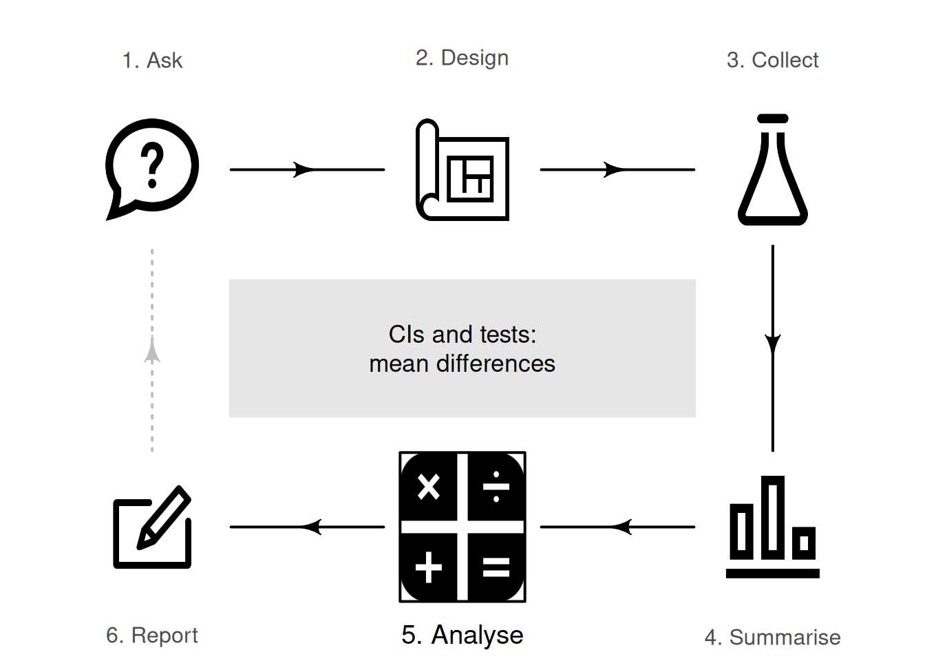
29 Mean differences (paired data): CIs and tests
You have learnt to ask an RQ, design a study, classify and summarise the data, construct confidence intervals, and conduct hypothesis tests. In this chapter, you will learn to:
- identify situations where mean differences are appropriate.
- construct confidence intervals for a mean difference.
- conduct hypothesis tests for the mean difference with paired data.
- determine whether the conditions for using these methods apply in a given situation.
29.1 Introduction: six-minute walk test
The six-minute walk test (6MWT) measures how far subjects can walk in six minutes, and is used as a simple, low-cost evaluation of fitness and other health-related measures. The recommended setting for the test is usually a walkway of at least \(30\,\text{m}\). Saiphoklang, Pugongchai, and Leelasittikul (2022) measured the 6MWT distance when the same subjects used both \(20\,\text{m}\) and \(30\,\text{m}\) walkways.
The comparison is within individuals (Sect. 2.4); this is a repeated-measures study. Each subject has a pair of 6MWT measurements, and the study produced paired data (below), the topic of this chapter.
Some differences are negative. This does not mean a negative distance. Since the differences are computed as the \(30\,\text{m}\) distance minus the \(20\,\text{m}\) distance, a negative difference means the \(20\,\text{m}\) distance is a larger value than the \(30\,\text{m}\) distance.
29.2 Paired data
The data above are paired. Computing the differences or changes between the pairs of observations makes sense, since the values for each pair belong to the same unit of analysis (the same person, in this case).
Pairing data, when appropriate, is useful because individuals can vary substantially, and pairing means that extraneous variables (potentially, confounding variables) are held constant for those paired observations. For example, each pair of measurements in the data above are recorded for the same person, so both measurements are recorded for someone of the same age, same sex, and with the same physical attributes.
Pairing is a form of blocking (Sect. 7.2). Pairing is a good design strategy when the individuals in the pair are the same, or are very similar, for many extraneous variables. (For example, the pair may comprise two different people, of the same sex, with similar age, height and weight.) Pairing often involves taking two measurements from the same individuals, as in the data above.
Definition 29.1 (Paired data) Paired data occurs when the outcome is compared for two different, distinct situations for each unit of analysis.
Paired studies appear in many situations; for example, when:
- heart rate is measured for each twin in a pair (the twin-pair is the 'individual'), one of whom exercises regularly and one who does not. Pairing the twins is reasonable, given the shared genetics (and probably childhood environments also). The difference between the hearts rates of the twins can be recorded for each pair.
- the body temperature of dogs (the 'individuals') is measured using both rectal and ear thermometers for each dog. The difference between the two recorded temperatures from the thermometers for each dog is recorded.
- blood pressure is recorded from some individuals (Group A) after receiving Drug A, and from another group of individuals (Group B) after receiving Drug B. Each person in Group A is matched with someone in Group B of the same sex, similar age and similar weight (e.g., in one of the pairs, both individuals are male, about \(30\) years-of-age, and weighing about \(95\,\text{kg}\)). The difference between the blood pressure measurements for the individual in Group A and the matched person in Group B is recorded for each pair.
- the number of campers is recorded at many national parks (the 'individuals') on the first weekend in summer, and on the first weekend in winter. The difference in camper numbers for each national park between these time points is recorded.
Many of these examples can be extended to beyond two measurements. For instance, temperatures can be compared on each dog using three different types of thermometers. In this chapter, only pairs of measurements are studied, and only for quantitative variables.
29.3 Summarising the data
For the 6MWT study, the distance is measured for the same subjects for two different walkway distances. Each subject receives two measurements, and the difference between the distances walked for each individual is computed.
Since the data are paired, an appropriate graph is a histogram of the differences (Sect. 13.3.1); specifically, \(30\,\text{m}\) distance minus the \(20\,\text{m}\) distance. A boxplot comparing 6MWT distance for both walkway lengths (that is, not pairing the data) shows the distribution of distances, and the median distances, are very similar (Fig. 29.1, left panel). Any difference in individuals' 6MWT distances is difficult to see and detect. In addition, linking the \(20\,\text{m}\) and \(30\,\text{m}\) distances that belong together for each individual patient is not possible.
However, using a histogram of the differences makes the individuals' differences easier to see (Fig. 29.1, right panel). The histogram also makes it easy to see that some subjects walked further with a \(20\,\text{m}\) walkway, and some further for a \(30\,\text{m}\) walkway. Individually graphing the distances for both walkway distances may also be useful too (e.g., using two histograms), but a graph of the differences is crucial, as the RQ is about those differences. A case-profile plot (Sect. 13.3.2) is also appropriate, but is difficult to read for these data because sample size is large (a line is needed for each of the \(50\) units of analysis).
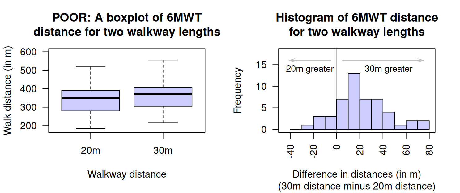
FIGURE 29.1: Plots of the 6MWT data. Left: graphing the data incorrectly as unpaired. Right: a histogram of 6MWT distances changes (\(30\,\text{m}\) walkway distance minus \(20\,\text{m}\) walkway distance; the vertical grey line represents no change in distance).
The 6MWT distances for each walkway length can be summarised individually (the first two rows of Table 29.1) using the methods of Chap. 23, using software (Fig. 29.2). All statistics are slightly different for the two walkway distances; in particular, the mean \(30\,\text{m}\) walkway distance is slightly larger. However, since the RQ is about the difference between the distances, a numerical summary of the differences is essential (third row of Table 29.1, based on Fig. 29.2). Notice that the third row of information is computed from the values in the Diff. column in the data above, not by (for instance) finding the difference between the standard deviations in the first two rows.
| Mean | Median | Std deviation | Std error | Sample size | |
|---|---|---|---|---|---|
| 20m walkway distance (in m) | \(337.82\) | \(351.0\) | \(71.801\) | \(10.154\) | \(50\) |
| 30m walkway distance (in m) | \(359.85\) | \(371.4\) | \(77.250\) | \(10.925\) | \(50\) |
| Difference (in m) | \(\phantom{0}22.03\) | \(\phantom{0}17.0\) | \(22.039\) | \(\phantom{0}3.117\) | \(50\) |
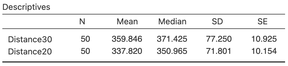
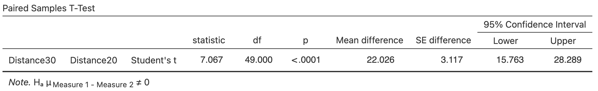
FIGURE 29.2: The 6MWT data: numerical summary software output for each group (top), and the CI and test results (bottom).
The differences (i.e., the Diff. column in the data given in Sect. 29.1) can be treated like a single sample of data (Table 29.2), with the notation adapted accordingly:
- \(\mu_d\): the mean difference in the population (in m).
- \(\bar{d}\): the mean difference in the sample (in m).
- \(s_d\): the sample standard deviation of the differences (in m).
- \(n\): the number of differences.
| One sample mean | Mean difference | |
|---|---|---|
| The observations: | Values: \(x\) | Differences: \(d\) |
| Population mean: | \(\mu\) | \(\mu_d\) |
| Sample mean: | \(\bar{x}\) | \(\bar{d}\) |
| Standard deviation: | \(s\) | \(s_d\) |
| Standard error of \(\bar{x}\): | \(\displaystyle\text{s.e.}(\bar{x}) = \frac{s}{\sqrt{n}}\) | \(\displaystyle\text{s.e.}(\bar{d}) = \frac{s_d}{\sqrt{n}}\) |
| Sample size: | Number of observations: \(n\) | Number of differences: \(n\) |
29.4 Confidence intervals for \(\mu_d\)
The data in Sect. 29.1 can be used to answer this repeated-measures, estimation RQ:
For Thai patients with chronic obstructive pulmonary disease, what is the mean difference between the 6MWT distance when subjects use a \(20\,\text{m}\) walkway and a \(30\,\text{m}\) walkway?
Every possible sample of \(n = 50\) subjects comprises different people, and hence produces different 6MWT distances for \(20\,\text{m}\) and \(30\,\text{m}\) walkways. For this reason, the 6MWT distance summaries in Table 29.1 include standard errors. Since the 6MWT distance varies from sample to sample for each person, the differences between the distances for each person varies from sample to sample too, and also have a sampling distribution.
Definition 29.2 (Sampling distribution of a sample mean difference) The sampling distribution of a sample mean difference is (when certain conditions are met; Sect. 29.6) described by:
- an approximate normal distribution,
- centred around the sampling mean whose value is the population mean difference \(\mu_d\),
- with a standard deviation, called the standard error of the difference, of \(\displaystyle\text{s.e.}(\bar{d}) = \frac{s_d}{\sqrt{n}}\),
where \(n\) is the number of differences, and \(s_d\) is the standard deviation of the individual differences in the sample.
For the 6MWT data, the sample mean differences \(\bar{d}\) are described by (Fig. 29.3):
- approximate normal distribution,
- with a sampling mean whose value is \(\mu_{{d}}\),
- with a standard error of \[\begin{equation} \text{s.e.}(\bar{d}) = \frac{22.039}{\sqrt{50}} = 3.117. \tag{29.1} \end{equation}\]
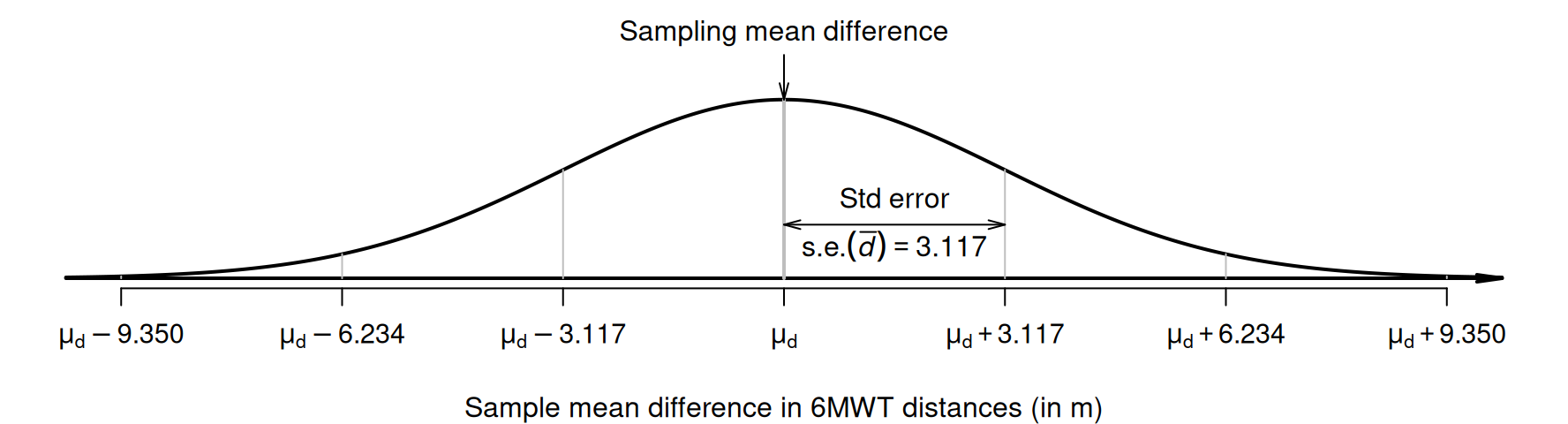
FIGURE 29.3: The sampling distribution is a normal distribution; it describes how the sample mean difference between the 6MWT distances varies in samples of size \(n = 50\).
The CI for the mean difference has the same form as for a single mean (Chap. 23). The \(95\)% confidence interval (CI) for \(\mu_d\) is \[ \bar{d} \pm \big(\text{multiplier} \times\text{s.e.}(\bar{d})\big). \] As usual when the sampling distribution has an approximate normal distribution, an approximate \(95\)% CI uses the approximate multiplier of \(2\) (from the \(68\)--\(95\)--\(99.7\) rule). This is the same as the CI for \(\bar{x}\) if the differences are treated as the data.
For the 6MWT data, the approximate \(95\)% CI is: \[ 22.03 \pm (2 \times 3.117), \] or \(22.03\pm 6.234\,\text{m}\) (so the margin of error is \(6.234\,\text{m}\)). Equivalently, the CI is from \(22.03 - 6.234 = 15.796\,\text{m}\), up to \(22.03 + 6.234 = 28.264\,\text{m}\). We write:
The mean difference in the 6MWT distances when using a \(20\,\text{m}\) and \(30\,\text{m}\) walkway is \(22.03\,\text{m}\) (\(\text{s.e.} = 3.117\); \(n = 50\)), with an approximate \(95\)% CI from \(15.80\,\text{m}\) to \(28.26\,\text{m}\), further for a \(30\,\text{m}\) walkway.
The CI means that the reasonable values for the population mean difference in 6MTW distances are between \(15.80\,\text{m}\) and \(28.26\,\text{m}\). Alternatively, we are \(95\)% confident that the population mean difference between the 6MWT distances is between \(15.80\,\text{m}\) and \(28.26\,\text{m}\) (further for \(30\,\text{m}\) walkway). A difference of this magnitude probably has practical importance. Also notice that the direction of the difference is given: 'further for \(30\,\text{m}\) walkway'.
Statistical software produces exact \(95\)% CIs, which may be slightly different from the approximate \(95\)% CI (recall: the \(68\)--\(95\)--\(99.7\) rule gives approximate multipliers). For the 6MWT data, the approximate and exact \(95\)% CIs are the same to one decimal place (Fig. 29.2). We write:
The mean difference in the 6MWT distances when using a \(20\,\text{m}\) and \(30\,\text{m}\) walkway is \(22.03\,\text{m}\) (\(\text{s.e.} = 3.117\); \(n = 50\)), with a \(95\)% CI from \(15.76\,\text{m}\) to \(28.29\,\text{m}\) further for a \(30\,\text{m}\) walkway.
29.5 Hypothesis tests for \(\mu_d\): \(t\)-test
The data in Sect. 29.1 can be used to answer this repeated-measures, decision-making RQ:
For Thai patients with chronic obstructive pulmonary disease, is there a mean increase in 6MWT distance using a \(30\,\text{m}\) walkway compared to a \(20\,\text{m}\) walkway?
In Sect. 29.1, the differences were defined as the \(30\,\text{m}\) distance minus the \(20\,\text{m}\) distance, which is consistent with the wording in this RQ. This RQ asks if the mean walking distance is, in general, a smaller value when subjects use a \(20\,\text{m}\) walkway compared to a \(30\,\text{m}\) walkway (that is how positive differences eventuate). The parameter is the population mean difference in 6MWT, \(\mu_d\). Note that the RQ is worded as one-tailed.
The null hypothesis is that 'there is no mean change in 6MWT, in the population':
- \(H_0\): \(\mu_d = 0\).
This hypothesis, which we initially assume to be true, postulates that the mean reduction may not be zero in the sample, due to sampling variation.
Since the RQ asks specifically if the mean distance is smaller for a \(20\,\text{m}\) walkway, the alternative hypothesis is one-tailed (Sect. 28.2). According to how the differences have been defined, the alternative hypothesis is:
- \(H_1\): \(\mu_d > 0\) (i.e., one-tailed).
This hypothesis says that the mean change in the population is greater than zero, because of the wording of the RQ, and because of how the differences were defined. If the differences were defined in the opposite way (as 'the \(20\,\text{m}\) distance minus the \(30\,\text{m}\) distance') then the alternative hypothesis would be \(\mu_d < 0\), which has the same meaning.
The sampling distribution, as described in Sect. 29.2, still applies, where \(\mu_d\) is assumed to be the value given in \(H_0\) (see Fig. 29.4):
- an approximate normal distribution,
- centred around the sampling mean whose value is the population mean difference \(\mu_d = 0\) (from \(H_0\)),
- with a standard deviation of \(\displaystyle\text{s.e.}(\bar{d}) = 3.117\) (from Equation (29.1)).
The sample mean difference can be located on the sampling distribution by computing the \(t\)-score: \[ t = \frac{\bar{d} - \mu_{d}}{\text{s.e.}(\bar{d})} = \frac{22.026 - 0}{3.117} = 7.07, \] following the ideas in Equation (27.2). Software displays the same \(t\)-score (Fig. 29.2). This is a huge \(t\)-score.
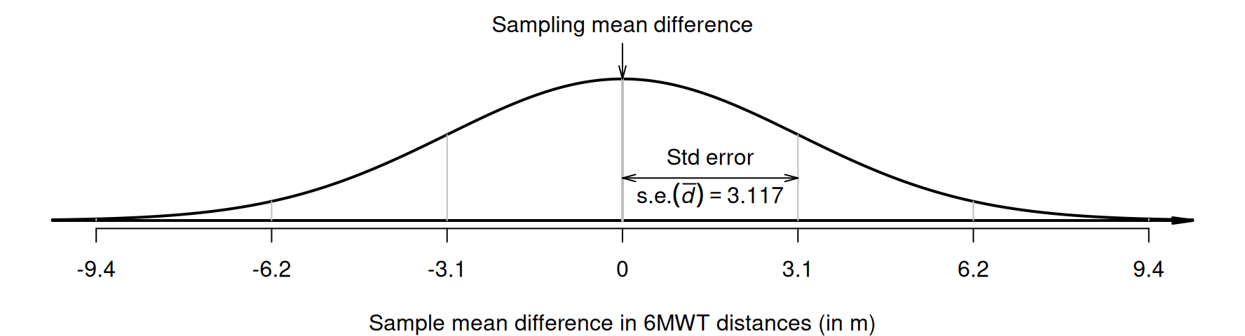
FIGURE 29.4: The sampling distribution is a normal distribution; it describes how the sample mean difference between the 6MWT distances varies in samples of size \(n = 50\).
A \(P\)-value determines if the sample data are consistent with the assumption (Table 28.1). Since \(t = 7.07\), and since \(t\)-scores are like \(z\)-scores, the one-tailed \(P\)-value will be very small (based on the \(68\)--\(95\)--\(99.7\) rule). Software (Fig. 29.2) reports that the two-tailed \(P\)-value is less than \(0.0001\). Hence, the one-tailed \(P\)-value is less than \(0.0001/2 = 0.00005\).
The software clarifies how the differences have been computed.
At the left of the output (Fig. 29.2), the order implies the differences are found as Dist30 (the \(30\,\text{m}\) walk distance) minus Dist20 (the \(20\,\text{m}\) walk distance), the same as our definition.
The one-tailed \(P\)-value is less than \(0.00005\), suggesting very strong evidence (Table 28.1) to support \(H_1\). A conclusion requires an answer to the RQ, a summary of the evidence leading to that conclusion, and some summary statistics:
Very strong evidence exists in the sample (paired \(t = 7.07\); one-tailed \(P < 0.0005\)) of a mean reduction in 6MWT for a \(20\,\text{m}\) walkway compared to a \(30\,\text{m}\) walkway (mean reduction: \(22.03\,\text{m}\); \(95\)% CI: \(15.76\,\text{m}\) to \(28.29\,\text{m}\); \(n = 50\)).
Note that the direction of the difference is provided.
Saying 'there is evidence of a difference' is insufficient. You must state which measurement is, on average, higher (that is, what the differences mean).
29.6 Statistical validity conditions
As with any CI and hypothesis test, these results apply under certain conditions. The conditions under which the results are statistically valid for paired data are similar to those for one sample mean, rephrased for differences.
The CI and test for a mean difference is statistically valid if either of these is true:
- when \(n \ge 25\). (If the distribution of the differences is highly skewed, the sample size may need to be larger.)
- when \(n < 25\), and the sample data come from a population with a normal distribution.
The sample size of \(25\) is a rough figure; some books give other values (such as \(30\)).
This condition ensures that the distribution of the sample mean differences has an approximate normal distribution (so that, for example, the \(68\)--\(95\)--\(99.7\) rule can be used). Provided the sample size is larger than about \(25\), this will be approximately true even if the distribution of the differences in the population does not have a normal distribution. That is, when \(n \ge 25\) the sample mean differences generally have an approximate normal distribution, even if the differences themselves don't have a normal distribution. The units of analysis are also assumed to be independent (e.g., from a simple random sample).
If the statistical validity conditions are not met, other methods (e.g., non-parametric methods (Conover 2003); resampling methods (Efron and Hastie 2021)) may be used. For paired qualitative data, McNemar's test can be used (Conover 2003).
Example 29.1 (Statistical validity) For the 6MWT data, the sample size is \(n = 50\), so the results are statistically valid. Neither the differences in the population, nor the distances in the population for the individual walkway lengths, need to follow a normal distribution.
29.7 Example: invasive plants
Skypilot is an alpine wildflower native to the Colorado Rocky Mountains (USA). In recent years, a willow shrub (Salix) has been encroaching on skypilot territory and, because willow often flowers early, Kettenbach et al. (2017) studied whether the willow may 'negatively affect pollination regimes of resident alpine wildflower species' (p. \(6\,965\)).
Data for both species was collected at \(n = 25\) different sites, so the data are paired by site (Sect. 29.1). The data are shown in Sect. 13.4. The parameter is \(\mu_d\), the population mean difference in day of first flowering for skypilot, less the day of first flowering for willow. A positive value for the difference means that the skypilot values are larger, and hence that willow flowered first. The RQ is:
In the Colorado Rocky Mountains, is there a mean difference between first-flowering day for the native skypilot and encroaching willow?
The hypotheses are \[ \text{$H_0$: $\mu_d = 0$}\quad\text{and}\quad\text{$H_1$: $\mu_d\ne 0$}, \] where the alternative hypothesis is two-tailed, and \(\mu_d\) is the mean difference between first-flowering day for the native skypilot and encroaching willow.
Explaining how the differences are computed is important. The differences here are skypilot minus willow first-flowering days.
However, the differences could be computed as willow minus skypilot first-flowering days. Either is fine, as long as you remain consistent. The meaning of any conclusions will be the same.
The data are summarised graphically in Fig. 13.5 and numerically (Table 29.3, after rounding) using software output (Fig. 29.5).
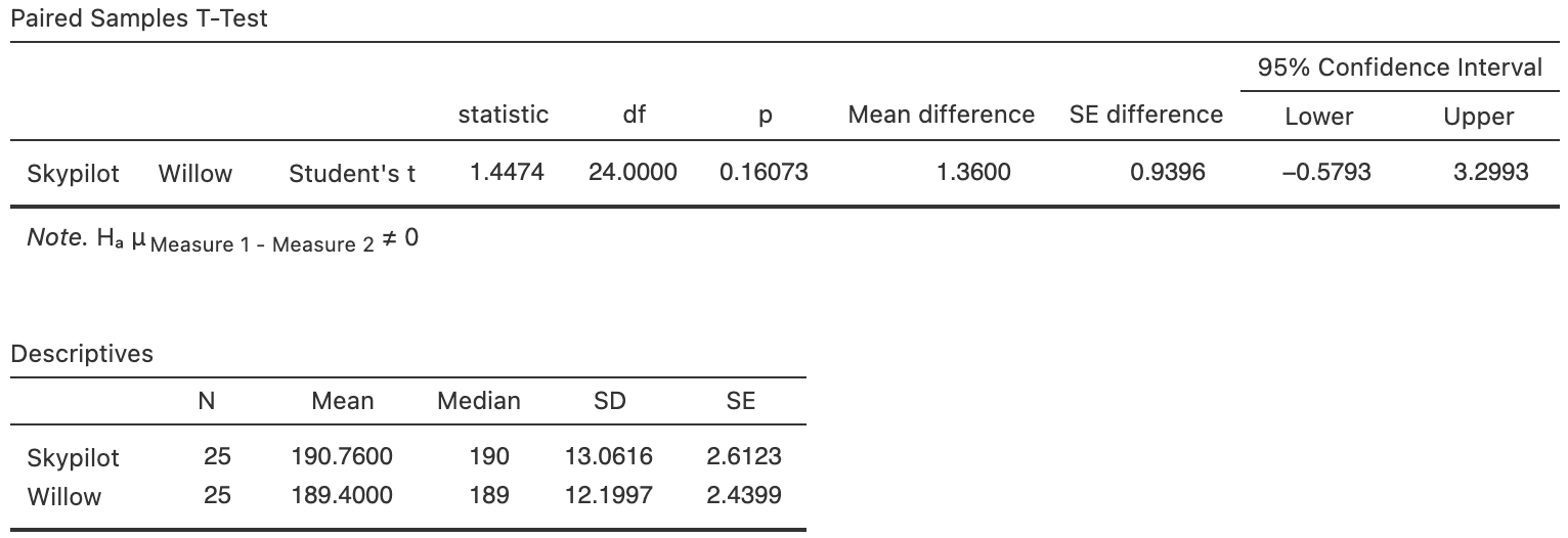
FIGURE 29.5: Software output for the flowering-day data.
| Mean | Standard deviation | Standard error | Sample size | |
|---|---|---|---|---|
| Willow (encroaching) | \(189.40\) | \(12.200\) | \(2.440\) | \(25\) |
| Skypilot (native) | \(190.76\) | \(13.062\) | \(2.612\) | \(25\) |
| Differences | \(\phantom{0}\phantom{0}1.36\) | \(\phantom{0}4.698\) | \(0.940\) | \(25\) |
The standard error of the mean difference is \(\text{s.e.}(\bar{d}) = 0.9396\) (Fig. 29.5 or Table 29.3). The sampling distribution for \(\bar{d}\) has a normal distribution, centred around \(\mu_d\) with a standard deviation of \(\text{s.e.}(\bar{d}) = 0.9396\).
The approximate \(95\)% CI for the mean difference is \[ 1.36 \pm ( 2\times 0.9396), \] or from \(-0.52\) to \(3.24\) days. The exact \(95\)% CI (Fig. 29.5) is \(-0.58\) to \(3.30\) days; the difference is because the approximate CI uses the approximate multiplier of \(2\) from the \(68\)--\(95\)--\(99.7\) rule.
The value of the test statistic (i.e., the \(t\)-score) is \[\begin{align*} t = \frac{\bar{d} - \mu_d}{\text{s.e.}(\bar{d})} = \frac{1.36 - 0}{0.9396} = 1.45, \end{align*}\] as in the output. This is a relatively small value of \(t\), so a large \(P\)-value is expected using the \(68\)--\(95\)--\(99.7\) rule. Indeed, the output shows that \(P = 0.161\): there is no evidence of a mean difference in first-flowering day (i.e., the sample mean difference could reasonably be explained by sampling variation if \(\mu_d = 0\)).
Since positive differences mean that willow flowers earlier, we write (using the exact CI):
No evidence exists (\(t = 1.45\); two-tailed \(P = 0.161\)) that the day of first-flowering is different for the encroaching willow and the native skypilot (mean difference: \(1.36\) days earlier for willow; approximate \(95\)% CI between \(0.52\) days earlier for skypilot to \(3.24\) days earlier for willow; \(n = 25\)).
The CI is statistically valid since \(n = 25\).
Be clear in your conclusion about how the differences are computed. Make sure to interpret the test and CI consistently with how the differences are defined.
We do not say whether the evidence supports the null hypothesis. We assume the null hypothesis is true, so we state how strong the evidence is to support the alternative hypothesis. The current sample presents no evidence to contradict the assumption (but future evidence may emerge).
29.8 Example: chamomile tea
Rafraf, Zemestani, and Asghari-Jafarabadi (2015) studied patients with Type 2 diabetes mellitus (T2DM). They randomly allocated \(32\) patients into a control group (who drank hot water), and another \(32\) patients to receive chamomile tea (p. 164):
The study was blinded so that the allocation of the intervention or control group was concealed from the researchers and statistician [...] The intervention group (\(n = 32\)) consumed one cup of chamomile tea [...] three times a day immediately after meals (breakfast, lunch, and dinner) for \(8\) weeks. The control group (\(n = 32\)) consumed an equivalent volume of warm water during the \(8\)-week period...
The total glucose (TG) was measured for each individual both before the intervention and after eight weeks on the intervention (a within-individuals comparison)}, in both the control and treatment groups (a between-individuals comparison)}. The data are not available, so no graphical summary of the data can be produced; however, the article gives a data summary (motivating Table 29.4).
| \(n\) | Mean | Std dev. | Mean | Std dev. | Mean | Std dev. | Std error | |
|---|---|---|---|---|---|---|---|---|
| Chamomile tea | \(\phantom{0}32\) | \(\phantom{0}203.00\) | \(\phantom{0}54.96\) | \(\phantom{0}164.37\) | \(\phantom{0}50.70\) | \(\phantom{0}38.62\) | \(\phantom{0}30.37\) | \(\phantom{0}\phantom{0}5.37\) |
| Control | \(\phantom{0}32\) | \(\phantom{0}178.25\) | \(\phantom{0}53.06\) | \(\phantom{0}185.37\) | \(\phantom{0}52.59\) | \(\phantom{0}{-7.12}\) | \(\phantom{0}36.66\) | \(\phantom{0}\phantom{0}6.48\) |
| Difference | \(\phantom{0}\phantom{0}24.75\) | \(\phantom{0}\phantom{0}21.00\) | \(\phantom{0}45.74\) |
Is there a mean reduction in TG in either group? Estimates of the mean reduction in each group can be found by constructing a CI for each group. First, the standard errors for each reduction are needed:
- \(\text{s.e.}(\bar{d}) = 30.37/\sqrt{32} = 5.37\).
- \(\text{s.e.}(\bar{d}) = 36.66/\sqrt{32} = 6.48\).
Then the approximate \(95\)% CIs are:
- \(38.62\pm (2\times 5.37)\), or from \(27.88\) to \(49.36\,\text{mg}.\text{dL}^{-1}\).
- \(-7.12\pm (2\times 6.48)\), or from \(-20.08\) to \(5.84\,\text{mg}.\text{dL}^{-1}\).
(A negative reduction in TG means an increase in TG.) The first CI suggests that the population mean difference is almost certainly larger than zero; the second suggests that a population mean difference of zero could reasonably have produced the sample data.
Of course, the sample mean differences in TG may be non-zero due to sampling variation. So, the following repeated-measures RQs can be asked:
- For patients with T2DM, is there a mean change in TG after eight weeks drinking chamomile tea?
- For patients with T2DM, is there a mean change in TG after eight weeks drinking hot water?
Then, the hypotheses are (where \(\mu_d\) represent the mean change in TG (in mg.dL\(-1\)) after eight weeks):
- \(H_0\): \(\mu_d = 0\) vs \(H_1\): \(\mu_d \ne 0\).
- \(H_0\): \(\mu_d = 0\) vs \(H_1\): \(\mu_d \ne 0\).
The two test statistics are: \[ t_T = \frac{38.62 - 0}{5.37} = 7.19\qquad\text{and}\qquad t_W = \frac{-7.12 - 0}{6.48} = -1.10, \] where the subscripts \(T\) and \(W\) refer to the tea and hot-water groups respectively. The \(t\)-score for the tea-drinking group is huge, so the two-tailed \(P\)-value will be very small using the \(68\)--\(95\)--\(99.7\) rule, and certainly smaller than \(0.001\). This means that there is evidence that chamomile tea had an impact on the mean change in TG.
In contrast, the \(t\)-score for the water-drinking group is small, so the two-tailed \(P\)-value will be large using the \(68\)--\(95\)--\(99.7\) rule, and certainly larger than \(0.10\). This means there is no evidence that placebo treatment (hot water) had any impact on mean change in TG (as one might expect for a placebo).
We write:
There is very strong evidence (\(t = 7.19\); two-tailed \(P < 0.001\)) of a mean change in TG for the chamomile-drinking groups (mean reduction: \(38.62\,\text{mg}.\text{dL}^{-1}\); approx. \(95\)% CI: \(27.88\) to \(49.36\,\text{mg}.\text{dL}^{-1}\); \(n = 32\)), but no evidence (\(t = -1.10\); two-tailed \(P > 0.10\)) of a mean change in the hot-water drinking group (mean reduction: \(-7.12\,\text{mg}.\text{dL}^{-1}\); approx. \(95\)% CI: \(-20.08\) and \(5.84\,\text{mg}.\text{dL}^{-1}\); \(n = 32\)).
The intervals have a \(95\)% chance of straddling the population mean reduction in TG. The sample sizes are larger than \(25\), so the results are statistically valid.
These hypothesis tests have allowed decisions to be made about each group individually. However, the two groups ultimately need to be compared; this is considered in Sect. 30.8.
29.9 Chapter summary
To compute a confidence interval (CI) for a mean difference, compute the sample mean difference, \(\bar{d}\), and identify the sample size \(n\). Then compute the standard error, which quantifies how much the value of \(\bar{d}\) varies across all possible samples: \[ \text{s.e.}(\bar{d}) = \frac{ s_d }{\sqrt{n}}, \] where \(s_d\) is the sample standard deviation. The margin of error is (multiplier\({}\times{}\)standard error), where the multiplier is \(2\) for an approximate \(95\)% CI (using the \(68\)--\(95\)--\(99.7\) rule). Then the CI is: \[ \bar{d} \pm \left( \text{multiplier}\times\text{standard error} \right). \] The statistical validity conditions should also be checked.
These steps are used to test a hypothesis about a population mean difference \(\mu_d\).
- Write the null hypothesis (\(H_0\)) and the alternative hypothesis (\(H_1\)); initially assume the value of \(\mu_d\) in the null hypothesis to be true.
- Describe the sampling distribution, which describes what to expect from the sample mean difference based on this assumption: under certain statistical validity conditions, the sample mean difference varies with:
- an approximate normal distribution,
- with sampling mean whose value is the value of \(\mu_d\) (from \(H_0\)), and
- having a standard deviation of \(\displaystyle \text{s.e.}(\bar{d}) =\frac{s_d}{\sqrt{n}}\).
- Compute the value of the test statistic: \[ t = \frac{ \bar{d} - \mu}{\text{s.e.}(\bar{d})}, \] where \(\mu_d\) is the hypothesised value given in the null hypothesis.
- The \(t\)-value is like a \(z\)-score, and so an approximate \(P\)-value can be estimated using the \(68\)--\(95\)--\(99.7\) rule, or found using software. Use the \(P\)-value to make a decision, and write a conclusion.
- Check the statistical validity conditions.
The following short video may help explain some of these concepts:
29.10 Quick review questions
Bacho et al. (2019) compared joint pain in stroke patients receiving a supervised exercise treatment. The same participants (\(n = 34\)) were assessed before and after treatment. The mean improvement in joint pain after \(13\) weeks was \(1.27\) (with a standard error of \(0.57\)) measured using a standardised tool.
Are the following statements true or false?
- For paired data, the mean of the differences is treated like the mean of a single variable.
- An appropriate graph for displaying these data is a histogram of the differences.
- The population mean difference is denoted \(\mu_d\).
- The standard error of the sample mean difference is denoted \(s_d\).
- Only 'before and after' studies can be paired.
- The null hypothesis is about the population mean difference.
- The value of the test statistic is \(2.23\).
- The approximate value of the two-tailed \(P\)-value is very small.
- The 'test statistic' for this test is a \(t\)-score.
29.11 Exercises
Answers to odd-numbered exercises are given at the end of the book.
Exercise 29.1 Which (if any) of these scenarios are paired?
- Heart rate is measured for each individual when sitting and when standing. (Some individuals have their heart rate recorded first while sitting, and some first while standing.) Each person receives two measurements, and the difference in heart rate between sitting and standing is recorded.
- The mean protein concentrations were compared in sea turtles before and after being rehabilitated (March et al. 2018).
Exercise 29.2 Which (if any) of these scenarios are paired?
- The mean HDL cholesterol concentration is recorded for a group of males and a group of females, and the means compared.
- Heart rate was recorded for \(36\) people, both before and after exercise, to determine how much the average heart rate increases.
Exercise 29.3 A group of primary school children was asked to complete a certain task on both a personal computer (PC) and using a tablet computer.
If the differences were defined as the time to complete the task on the PC, minus the time to complete the same task on a tablet (one difference for each child), what do the differences mean?
Exercise 29.4 Suppose water quality was recorded \(500\,\text{m}\) upstream and \(500\,\text{m}\) downstream of \(28\) different copper mines.
If the differences were defined as the pH downstream minus the water pH upstream for each river, what do the differences mean?
Exercise 29.5 Suppose, in the example of Sect. 29.7, the differences were defined as the day of first flowering for willow, less the day of first flowering for skypilot. Write down, and interpret the meaning of, the approximate \(95\)% CI for the mean difference in first-flowering times.
Exercise 29.6 Suppose, in the example of Sect. 29.8, the differences were defined as increase in total glucose (TG). Write down, and interpret the meaning of the approximate \(95\)% CI for the mean increase in TG for the tea-drinking group.
Exercise 29.7 [Dataset: Fruit]
Mukherjee, Deb, and Devy (2019) studied the effect of rainfall on growing Chayote squash (Sechium edule).
They compared the size of the fruit in a year with normal rainfall (2015) compared to a dry year (2014) on \(24\) farms:
For Chayote squash grown in Bangalore, what is the mean difference in fruit weight between a normal and dry year?
Ten fruits were gathered from each farm in both years, and the average (mean) weight of the fruit recorded for the farm. Since the same farms are used in both years, the data are paired (below). Data is missing for Farm 20 in the dry year (2014), so there are \(n = 23\) differences.
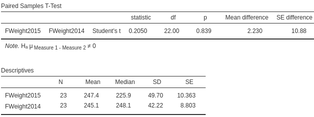
FIGURE 29.6: Software output for the fruit data.
- What is the unit of analysis? What is the units of observation?
- What is the advantage of using the same \(24\) farms twice each?
- Construct a suitable graph to display the differences.
- Create a numerical summary table for the data (use Fig. 29.6).
- What is the parameter? Carefully describe what it means.
- Write down the hypotheses.
- Sketch the sampling distribution.
- Compute the \(t\)-score.
- Determine the \(P\)-value.
- Construct an approximate \(95\)% CI for the mean difference in fruit weight.
- Are the test and the CI statistically valid?
- Write a conclusion.
Exercise 29.8 [Dataset: Captopril]
In a study of hypertension (Hand et al. 1996; MacGregor et al. 1979), \(n = 15\) patients were given a drug (Captopril) and their systolic blood pressure measured (in mm Hg) immediately before and two hours after being given the drug.
The aim is to see if there is evidence of a reduction in blood pressure after taking Captopril. Use the data (Table 13.5) and the software output (Fig. 29.7) to answer these questions.
- Explain why it is probably more sensible to compute differences as the Before minus the After measurements. What do the differences mean when computed this way?
- What is the advantage of using the same patients for both the before and after measurements, rather than one group for before measurements and a different group of people for after measurements?
- What is the parameter? Carefully describe what it means.
- Construct a suitable graph to display the differences.
- Write down the hypotheses.
- Sketch the sampling distribution.
- Write down the \(t\)-score.
- Write down the \(P\)-value.
- Write down the exact \(95\)% CI using the computer output (Fig. 29.7).
- Compute an approximate \(95\)% CI for the mean difference.
- Why are the two CIs different?
- Write a conclusion.
- Are the CI and test statistically valid?
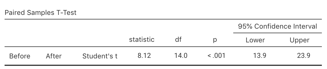
FIGURE 29.7: Software output for the Captopril data.
Exercise 29.9 People often struggle to eat the recommended intake of vegetables. Fritts et al. (2018) explored ways to increase vegetable intake in teens. Teens rated the taste of raw broccoli, and raw broccoli served with a specially-made dip.
Each teen (\(n = 100\)) had a pair of measurements: the taste rating of the broccoli with and without dip. Taste was assessed using a '\(100\,\text{mm}\) visual analogue scale', where a higher score means a better taste. In summary:
- for raw broccoli, the mean taste rating was \(56.0\) (with a standard deviation of \(26.6\));
- for raw broccoli served with dip, the mean taste rating was \(61.2\) (with a standard deviation of \(28.7\)).
Because the data are paired, the differences are the best way to describe the data. The mean difference in the ratings was \(5.2\), with standard error of \(3.06\).
- Construct a suitable numerical summary table.
- What does a positive difference mean?
- Perform a hypothesis test to see if the use of dip increases the mean taste rating.
- Compute the approximate \(95\)% CI for the mean difference in taste ratings.
- Are the CI and test statistically valid?
Exercise 29.10 Allen et al. (2018) examined the effect of exercise on smoking. Men and women were assessed on their 'intention to smoke', both before and after exercise for each subject (using two quantitative questionnaires). Smokers ('smoking at least five cigarettes per day') aged \(18\) to \(40\) were enrolled for the study. For the \(23\) women in the study, the mean intention to smoke after exercise reduced by \(0.66\) (with a standard error of \(0.37\)). (Larger values for 'intention to smoke' mean a greater intent to smoke.)
- Perform a hypothesis test to determine if there is evidence of a population mean reduction in intention-to-smoke for women after exercising.
- Find an approximate \(95\)% CI for the population mean reduction in intention to smoke for women after exercising.
- Are the CI and test statistically valid?
Exercise 29.11 [Dataset: Ferritin]
In a study (Cressie, Sheffield, and Whitford 1984) conducted at the Adelaide Children's Hospital (p. 107; emphasis added):
... a group of beta thalassemia patients [...] were treated by a continuous infusion of desferrioxamine, in order to reduce their ferritin content...
Using the data shown below, conduct a hypothesis test to determine if there is evidence that the treatment reduces the ferritin content, as intended. Make sure to include a \(95\)% CI in the conclusion.
| September | March | Reduction |
|---|---|---|
| \(\phantom{0}6630\) | \(\phantom{0}5100\) | \(\phantom{0}\phantom{0}1530\) |
| \(\phantom{0}4590\) | \(\phantom{0}3510\) | \(\phantom{0}\phantom{0}1080\) |
| \(\phantom{0}3510\) | \(\phantom{0}6600\) | \(\phantom{0}{-3090}\) |
| \(\phantom{0}6375\) | \(\phantom{0}8000\) | \(\phantom{0}{-1625}\) |
| \(\phantom{0}2500\) | \(\phantom{0}2800\) | \(\phantom{0}\phantom{0}{-300}\) |
| \(\phantom{0}1400\) | \(\phantom{0}2860\) | \(\phantom{0}{-1460}\) |
| \(\phantom{0}4580\) | \(\phantom{0}3640\) | \(\phantom{0}\phantom{0}\phantom{0}940\) |
| \(\phantom{0}6885\) | \(\phantom{0}9030\) | \(\phantom{0}{-2145}\) |
| \(\phantom{0}4200\) | \(\phantom{0}4420\) | \(\phantom{0}\phantom{0}{-220}\) |
| \(\phantom{0}5600\) | \(\phantom{0}7910\) | \(\phantom{0}{-2310}\) |
Exercise 29.12 [Dataset: Stress]
The concentration of beta-endorphins in the blood is a sign of stress.
Hoaglin, Mosteller, and Tukey (2011) measured the beta-endorphin concentration for \(19\) patients about to undergo surgery (Hand et al. 1996).
Each patient had their beta-endorphin concentrations measured \(12\)--\(14\,\text{h}\) before surgery, and also \(10\,\text{mins}\) before surgery (in fmol.mL\(-1\)).
A numerical summary (Table 29.6) was produced from output.
- Use the output to test the RQ.
- Use the software output in Fig. 29.8 to construct an approximate \(95\)% CI for the increase in beta-endorphin concentrations as surgery gets closer.
- Use the software output in Fig. 29.8 to write down the exact \(95\)% CI for the increase in beta-endorphin concentrations as surgery gets closer.
- Why is there a difference between the two CIs?
- Are the CI and test statistically valid?
| Means | Std.deviation | Std.Error | Sample.size | |
|---|---|---|---|---|
| 12--14 h before surgery | \(\phantom{0}8.35\) | \(\phantom{0}4.40\) | \(1.01\) | \(19\) |
| 10 min before surgery | \(16.05\) | \(12.51\) | \(2.87\) | \(19\) |
| Increase | \(\phantom{0}7.70\) | \(13.52\) | \(3.10\) | \(19\) |
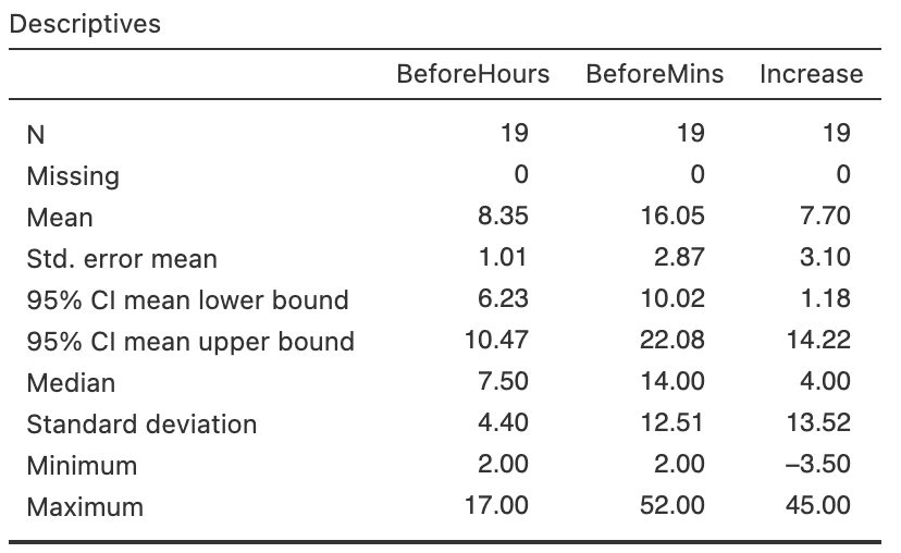
FIGURE 29.8: Software output for the surgery-stress data.
Exercise 29.13 A study of \(n = 213\) Spanish health students (Romero-Blanco et al. 2020) measured (among other variables) the number of minutes of vigorous physical activity (PA) performed by students weekly before and during the covid-19 lockdown (from March to April 2020 in Spain). Since the before and during lockdown were both measured on each participant, the data are paired. The data are summarised in Table 29.7.
- Explain what the differences mean.
- Compute the standard error of the differences.
- Perform a hypothesis test to determine if mean minutes of vigorous PA changed from before to during the lockdowns.
| Mean (mins) | Std dev. (mins) | |
|---|---|---|
| Before lockdown | \(28.47\) | \(54.13\) |
| During lockdown | \(30.66\) | \(30.04\) |
| Increase | \(\phantom{0}2.68\) | \(51.30\) |
Exercise 29.14 What happens when students start university? Many students will be responsible for their own meals for the first time, so some may forgo healthy foods for convenient, but less healthy, foods. Alternatively, some may not be able to afford sufficient or healthy food. Exercise regimes may also change.
D. A. Levitsky, Halbmaier, and Mrdjenovic (2004) recorded some students' weights as they began university, and then the same students' weight some later time. They asked the RQ:
For Cornell University students, what is the mean weight change in students after \(12\) weeks at university?
The data collected to answer this RQ are shown below (D. Levitsky 2023).
- Use the software output (Fig. 29.9) to compute an approximate \(95\)% CI for the weight gain from Weeks \(1\) to \(12\).
- Use the software output to write down an exact \(95\)% CI for the weight gain from Weeks \(1\) to \(12\).
- Comment on the two CIs.
- Are the CIs statistically valid?
- Conduct a hypothesis tests to determine if there is a change in mean weight from Weeks \(1\) to \(12\).
- Do you think the weight gain would be of practical importance?
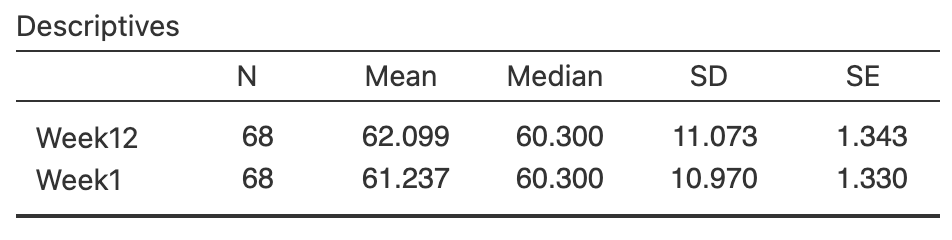
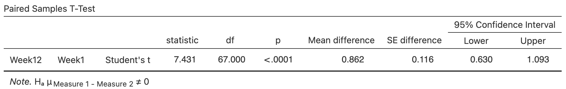
FIGURE 29.9: The weight-gain data: software output.
Exercise 29.15 [Dataset: Anorexia]
Young girls with anorexia (\(n = 29\)) received cognitive behavioural treatment (Hand et al. (1996)), and their weight before and after treatment were recorded.
In summary:
- Before the treatment, the mean weight was \(82.69\) pounds (\(s = 4.845\) pounds);
- After the treatment, the mean weight was \(85.70\) pounds (\(s = 8.352\) pounds).
The mean weight gain per girls was \(3.01\) pounds, with a standard deviation of \(7.31\) pounds. Find an approximate \(95\)% CI for the population mean weight gain. Do you think the treatment had any meaningful impact on the mean weight gain of the girls, based solely on these data?
Exercise 29.16 [Dataset: SoilCN]
Lambie, Mudge, and Stevenson (2021) compared the percentage nitrogen (%N) in soils from intensively-grazed irrigated and non-irrigated pastures.
The researchers paired similar irrigated and non-irrigated sites (p. 338):
The irrigated and non-irrigated pairs within each site were within \(100\,\text{m}\) of each other and were on the same soil, landform and usually the same farm with the same farm management...
One RQ in the study was:
For intensively grazed pastures sites, is there a mean reduction in percentage soil nitrogen (%N) when sites are irrigated, compared to non-irrigated?
The data are shown in the table below. Use the data to answer the RQ.
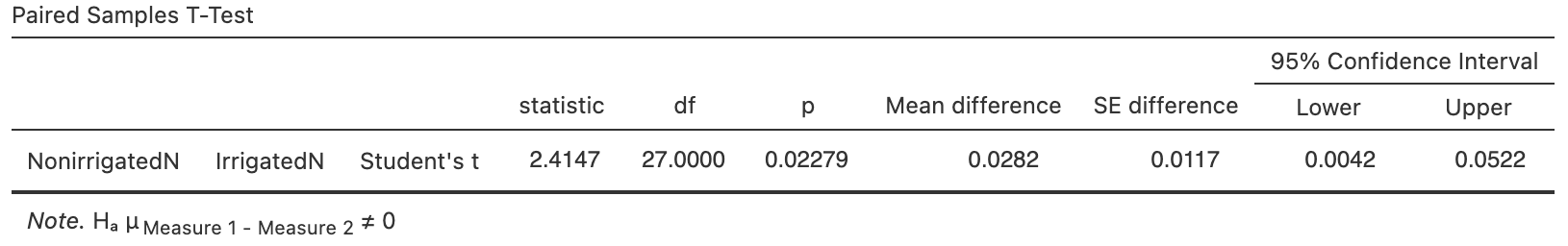
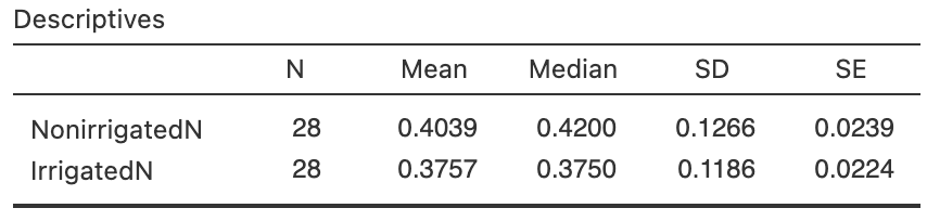
FIGURE 29.10: Software output for the nitrogen data. In the top table, the difference is implied as non-irrigated minus irrigated.
Exercise 29.17 [Dataset: Jumping]
Hébert-Losier, Boswell-Smith, and Hanzlı́ková (2023) recorded double-legged jumping distance for \(80\) healthy people, when they wore both shoes and were barefoot (Exercise 13.7).
Use the data to form a \(95\)% CI to estimate the mean distance people can jump further when barefoot.
Exercise 29.18 [Dataset: WCTennis]
Alberca et al. (2022) recorded the push time (the time between a shot and resetting) for French wheelchair tennis players, while holding a racquet and not holding a racquet (Table 13.8; Alberca (2022)).
Use the data to form a \(95\)% CI to estimate the mean difference between push times with and without a racquet.