27 Hypothesis tests: one mean

You have learnt to ask an RQ, design a study, classify and summarise the data, construct confidence intervals, and perform a hypothesis test for one proportion. In this chapter, you will learn to:

• identify situations where conducting a test for a mean is appropriate.
• conduct hypothesis tests for one sample mean, using a $t$-test.
• determine whether the conditions for using these methods apply in a given situation.

27.1 Introduction: body temperatures

The average internal body temperature is commonly believed to be $37.0$^oC ($98.6$^oF). This value is based on data over $150$ years old (Wunderlich 1868). Since then, the methods for measuring internal body temperature have changed substantially:

Thermometers used by Wunderlich were cumbersome, had to be read in situ, and, when used for axillary measurements [i.e., under the armpit]... required $15$ to $20\,\text{mins}$ to equilibrate. Today's thermometers are smaller and more reliable and equilibrate more rapidly. In addition, the mouth and rectum have replaced the axilla [armpit] as the preferred sites for monitoring body temperature.

--- Mackowiak, Wasserman, and Levine (1992), p. 1579

For this reason, the reported internal body temperature (recorded by newer instruments, in different locations) may have changed since the 1860s. Therefore, we could ask:

Is the population mean internal body temperature equal to $37.0$^oC?

A decision is sought about the value of the population mean body temperature. Presumably, the intended population is all people, though the population, in practice, may depend on what population is represented by the available data.

The population mean internal body temperature will never be known: the internal body temperature of every person alive would need to be measured, and even those not yet born. A sample must be studied.

Define the parameter as $\mu$, the population mean internal body temperature (in ^oC). A sample of people can be used to determine if evidence exists that the population mean internal body temperature is not $37.0$^oC, using the decision-making process (Sect. 25.3).

27.2 Assumptions: hypotheses

Step 1 of the decision-making process is to assume a value for the parameter. The established claim is that the population mean internal body temperature is $37.0$^oC, so we assume this value. This assumption becomes the null hypothesis: $$\text{$H_0$: } \mu = 37.0.$$ If the sample mean is not $37.0$^oC, this hypothesis proposes that the discrepancy is due to sampling variation.

The RQ asks if the population mean internal body temperate $\mu$ is equal to $37.0$^oC, or if it has changed. The RQ does not specifically ask if $\mu$ is smaller than $37.0$^oC, or larger than $37.0$^oC. This means the alternative hypothesis is two-tailed: $$\text{$H_1$: } \mu \ne 37.0.$$

27.3 Expectations: sampling distribution for $\bar{x}$

Step 2 of the decision-making process is to describe what values of the statistic (in this case, the sample mean $\bar{x}$) can be expected if the value of $\mu$ is assumed to be $37.0$ (the value specified in $H_0$). In other words, the sampling distribution of $\bar{x}$ needs to be described.

The sample mean varies from sample to sample, and varies with a normal distribution (whose standard deviation is called the standard error) under certain conditions (given in Sect. 27.8). The sampling distribution of $\bar{x}$ was described in Sect. 23.3, and repeated below.

Definition 27.1 (Sampling distribution of a sample mean) When the population standard deviation is unknown, the sampling distribution of the sample mean is (when certain conditions are met; Sect. 23.5) described by:

• an approximate normal distribution,
• centred around a sampling mean whose value is $\mu$,
• with a standard deviation (called the standard error of the mean), denoted $\text{s.e.}(\bar{x})$, whose value is $$\begin{equation} \text{s.e.}(\bar{x}) = \frac{s}{\sqrt{n}}, \tag{27.1} \end{equation}$$ where $n$ is the size of the sample, and $s$ is the sample standard deviation of the observations.

The mean of this sampling distribution---the sampling mean---has the value $\mu$. The standard deviation of this sampling distribution is called the standard error of the sample means, denoted $\text{s.e.}(\bar{x})$. When the population standard deviation $\sigma$ is unknown, the value of the standard error happens to be (see Equation (27.1)) $$\text{s.e.}(\bar{x}) = \frac{s}{\sqrt{n}}.$$

Mackowiak, Wasserman, and Levine (1992) gathered body-temperature data for $n = 130$ people, collated by Shoemaker (1996) (Fig. 27.1; Fig. 27.2). The data all come from

... volunteers participating in Shigella vaccine trials conducted at the University of Maryland Center for Vaccine Development, Baltimore...

--- Mackowiak, Wasserman, and Levine (1992), p. 1578

Hence, the population for the study (and RQ) should be redefined accordingly. From software output (Fig. 27.3), the sample mean is $\bar{x} = 36.8052$^oC and the sample standard deviation is $s = 0.4073$^oC. Using this value of $s$, the sampling distribution of $\bar{x}$ can be described, if $\mu$ really was $37.0$:

• an approximate normal distribution,
• with a sampling mean whose value is $\mu = 37.0$ (from $H_0$),
• with a standard deviation of $\text{s.e.}(\bar{x}) = s/\sqrt{n} = 0.4073/\sqrt{130} = 0.0357$ (as in the output).

Show 102550100 entries

	BodyTemp	Gender	HeartRate	BodyTempC
1	96.3	1	70	35.722
2	96.7	1	71	35.944
3	96.9	1	74	36.056
4	97	1	80	36.111
5	97.1	1	73	36.167
6	97.1	1	75	36.167
7	97.1	1	82	36.167
8	97.2	1	64	36.222
9	97.3	1	69	36.278
10	97.4	1	70	36.333

Showing 1 to 10 of 130 entries

Previous12345…13Next

FIGURE 27.1: The body temperature data.

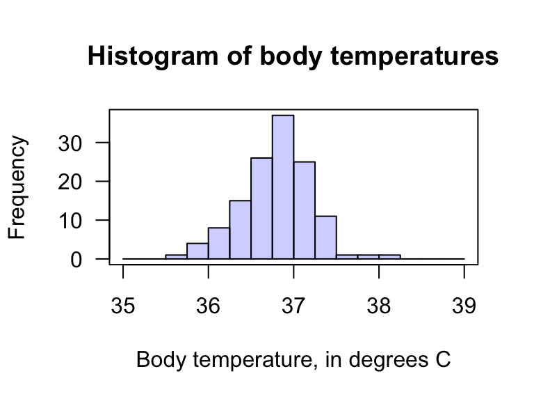
FIGURE 27.2: The histogram of the body temperature data.

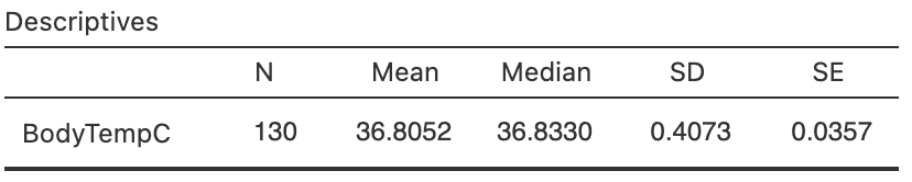
FIGURE 27.3: The software output summary for the body temperature data.

A picture of this sampling distribution (Fig. 27.4) shows how the sample mean varies when $n = 130$, for all possible samples when $\mu = 37.0$. For example, the value of $\bar{x}$ will be larger than $37.0357$^oC about $16$% of the time (using the $68$--$95$--$99.7$ rule) if $\mu$ really is $37.0$.

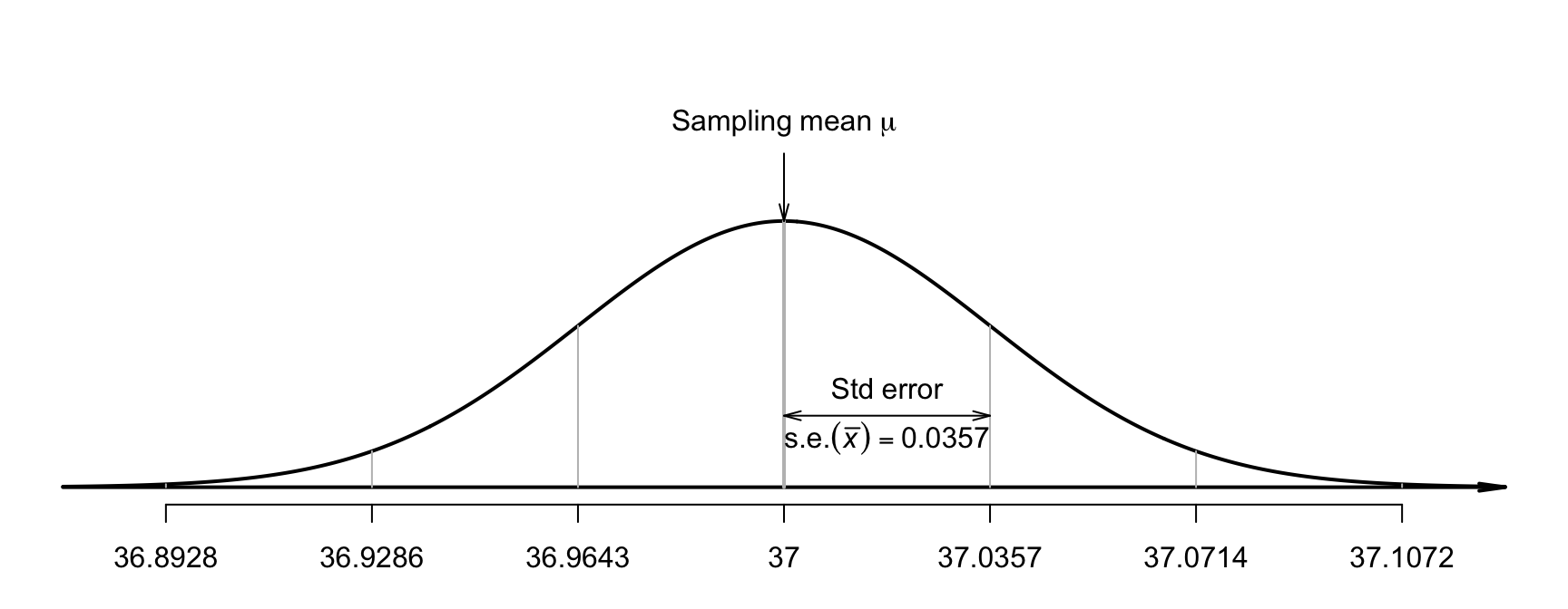
FIGURE 27.4: The distribution of sample mean body temperatures, if the population mean is $37.0^\circ$C and $n = 130$. The grey vertical lines are $1$, $2$ and $3$ standard deviations from the mean.

27.4 Observations: $t$-score

Step 3 of the decision-making process is to evaluate the observations. Locating $\bar{x} = 36.8052$ on the sampling distribution (Fig. 27.5) shows that this observed sample mean is, relatively speaking, extremely low: a sample mean this low is very unlikely to occur in any sample of $n = 130$ when $\mu = 37.0$. How many standard deviations is $\bar{x}$ away from $\mu = 37.0$? Compute: $$\frac{\text{statistic} - \text{mean of the distribution}}{\text{std dev. of the distribution}} = \frac{36.8052 - 37.0}{0.035724} = -5.453.$$ This is like a $z$-score: it measures the number of standard deviations that the value is from the mean. However, it is not a $z$-score; it is a $t$-score. Both $t$- and $z$-scores measure the number of standard deviations that a value is from the mean. Here the value is a $t$-score, because the population standard deviation $\sigma$ is unknown, and the sample standard deviation is used instead to compute $\text{s.e.}(\bar{x})$.

Like $z$-scores, $t$-scores measure the number of standard deviations that a value is from the mean of the distribution.

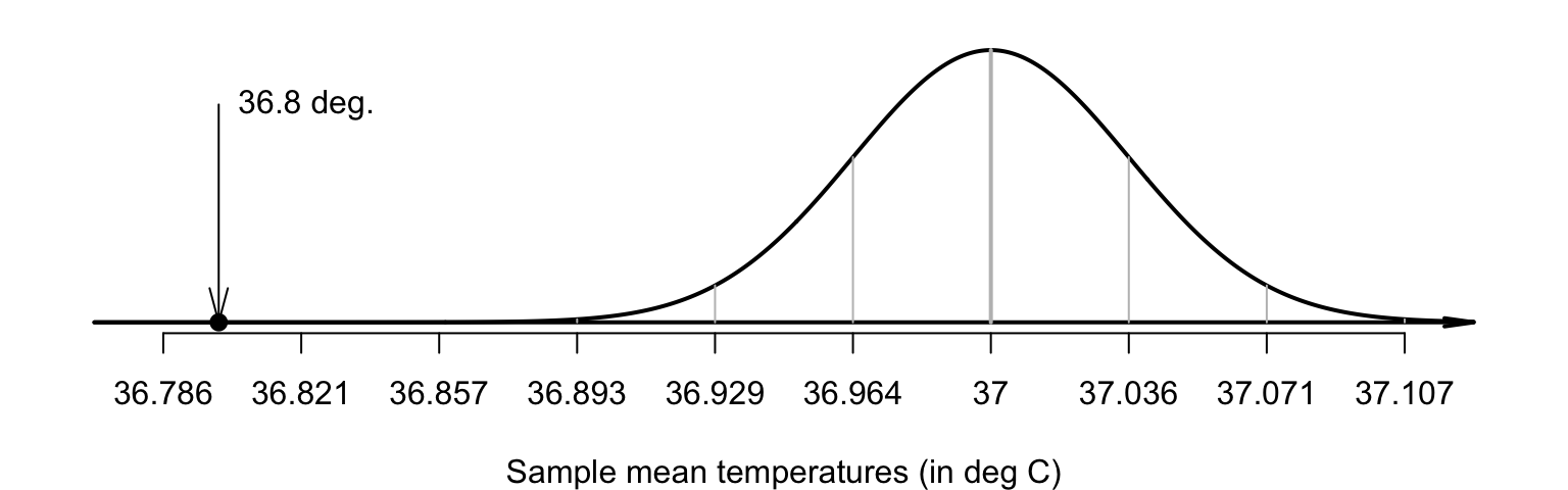
FIGURE 27.5: The sample mean of $\bar{x} = 36.8041^\circ$C is very unlikely to be observed in any sample of size $n = 130$, if $\mu = 37.0^\circ$C.The standard deviation of the distribution is $\text{s.e.}(\bar{x}) = 0.035724$.

The calculation is therefore: $$t = \frac{36.8052 - 37.0}{0.035724} = -5.453.$$ The observed sample mean is more than five standard deviations below the population mean, which is highly unusual based on the $68$--$95$--$99.7$ rule (Fig. 27.5). This is very persuasive evidence that $\mu$ is not $37.0$.

In general, when the sampling distribution has an approximate normal distribution and the sample standard deviation is used to compute the standard error, the $t$-score is $$\begin{equation} t = \frac{\text{sample statistic} - \text{mean of the sampling distribution}} {\text{standard error of the sampling distribution}} = \frac{\bar{x} - \mu}{\text{s.e.}(\bar{x})}. \tag{27.2} \end{equation}$$

27.5 Decision: $P$-value

As seen in Sect. 26.7, a $P$-value quantifies how unusual the observed sample statistic is, after assuming $H_0$ is true. Since $t$-scores and $z$-scores are very similar, the $P$-value can be approximated using the $68$--$95$--$99.7$ rule and a diagram, or approximated using $z$-tables (Appendix B.1). Usually, however, software is used to compute the $P$-value. $t$-scores and $z$-scores with the same value produce almost the same $P$-values, except for small sample sizes.

Both methods produce approximate $P$-values only, since the approximations are based on using $z$-scores rather than $t$-scores. Usually, software is used to determine precise $P$-values for $t$-scores (Fig. 27.6). The output (under the heading p) shows that the $P$-value is indeed very small: less than $0.001$ (written $P < 0.001$).

Some software reports a $P$-value of 0.000, which really means that the $P$-value is zero to three decimal places. Since $P$-values can never be exactly zero, we should write $P < 0.001$: that is, the $P$-value is smaller than $0.001$.

This $P$-value means that, if $\mu = 37.0$, a sample mean as low as $36.8052$ would be very unusual to observe (from a sample size of $n = 130$). And yet, we did. Using the decision-making process, this implies that the initial assumption (i.e., $H_0$) is contradicted by the data: we observed something extremely unlikely if $\mu = 37.0$. That is, there is very persuasive evidence that the population mean body temperature is not $37.0$^oC.

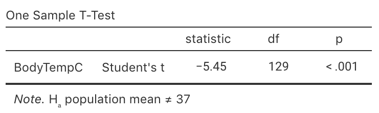
FIGURE 27.6: Software output for conducting the $t$-test for the body temperature data.

For one-tailed tests, the $P$-value is half the value of the two-tailed $P$-value.

As seen in Sect. 26.7, $P$-values measure the probability of observing the sample statistic (or something more extreme), assuming the population parameter is the value given in $H_0$. For the body-temperature data then, where $P < 0.001$, the $P$-value is very small, so very strong evidence exists that the population mean body temperature is not $37.0$^oC.

27.6 Writing conclusions

Communicating the results of any hypothesis test requires an answer to the RQ, a summary of the evidence used to reach that conclusion (such as the $t$-score and $P$-value, stating if the $P$-value is one- or two-tailed), and some sample summary information (including a CI). For the body-temperature example, write:

The sample provides very strong evidence ($t = -5.45$; two-tailed $P < 0.001$) that the population mean body temperature is not $37.0$^oC ($\bar{x} = 36.81$; $95$% CI: $36.73$ to $36.88$^oC; $n = 130$).

This statement contains the three components.

1. The answer to the RQ: the sample provides very strong evidence that the population mean body temperature is not $37.0$^oC. The alternative hypothesis is two-tailed, so the conclusion is that the population mean body temperature is not equal to  $37.0$^oC.
2. The evidence used to reach the conclusion: $t = -5.45$; two-tailed $P < 0.001$.
3. Some sample summary information: the sample mean (with the CI) and the sample size.

The test is about the mean internal body temperature; individuals have internal body temperatures ranging from $35.722$^oC to $38.222$^oC.

The difference between the value of $37.0$^oC and the sample mean of $36.81$^oC is small in absolute terms, and is probably of little practical importance for most applications. Notice that the CI does not include the value of $\mu = 37.0$.

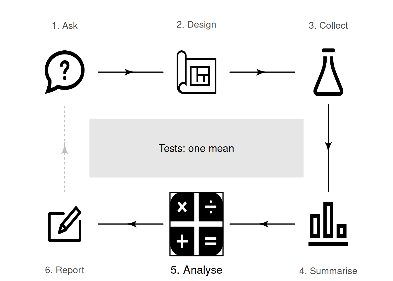
27.7 Process overview

Let's recap the decision-making process for this body temperatures (Fig. 27.7) example:

1. Assumption. Write the null hypothesis about the parameter (based on the RQ): $H_0$: $\mu = 37.0$. In addition, write the alternative hypothesis: $H_1$: $\mu \ne 37.0$. (This alternative hypothesis is two-tailed.)
2. Expectation. The sampling distribution describes what to expect from the statistic if the null hypothesis is true. The sampling distribution is an approximate normal distribution.
3. Observation. Compute the $t$-score: $t = -5.45$. The $t$-score can be computed by software, or using the general equation in Equation (27.2).
4. Decision. Determine if the data are consistent with the assumption, by computing the $P$-value. Here, the $P$-value is much smaller than $0.001$. The $P$-value can be computed by software, or approximated using the $68$--$95$--$99.7$ rule. The conclusion is that there is very strong evidence that $\mu$ is not $37.0$.

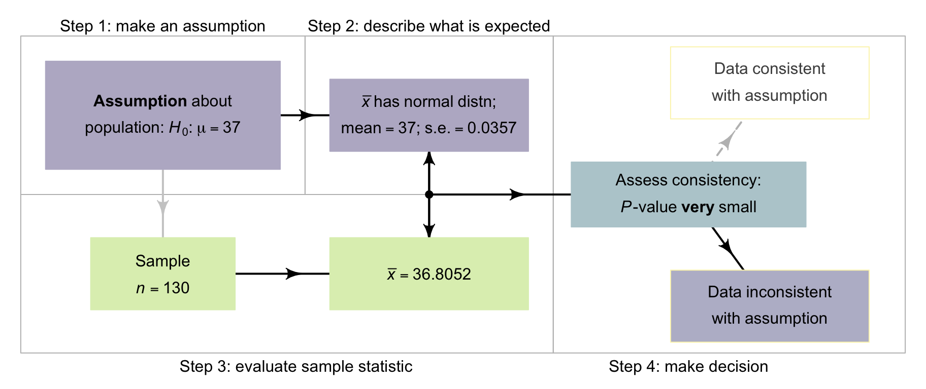
FIGURE 27.7: The decison-making process for the body-temperature data.

27.8 Statistical validity conditions

All hypothesis tests have underlying conditions to be met so that the results are statistically valid. For a test of one mean, this means that the sampling distribution must have an approximate normal distribution so that $P$-values can be found.

The test for a single mean is statistically valid if either of these is true:

• when $n \ge 25$. (If the distribution of the data is highly skewed, the sample size may need to be larger.)
• when $n < 25$, and the sample data come from a population with a normal distribution.

The sample size of $25$ is a rough figure; some books give other values (such as $30$).

This condition ensures that the distribution of the sample means has an approximate normal distribution (so that, for example, the $68$--$95$--$99.7$ rule can be used). Provided the sample size is larger than about $25$, this will be approximately true even if the distribution of the individuals in the population does not have a normal distribution. That is, when $n \ge 25$ the sample means generally have an approximate normal distribution, even if the data themselves do not have a normal distribution. The units of analysis are also assumed to be independent (e.g., from a simple random sample).

If the statistical validity conditions are not met, other similar options include a sign test or a Wilcoxon signed-rank test (Conover 2003), or using resampling methods (Efron and Hastie 2021).

Example 27.1 (Statistical validity) The hypothesis test regarding body temperature is statistically valid since the sample size is larger than $25$ ($n = 130$). (The data, as displayed in Fig. 27.2, do not need to come from a population with a normal distribution.)

27.9 Example: student IQs

Standard IQ scores are designed to have a mean in the general population of $\mu = 100$. Researchers at Griffith University (GU) asked:

For students at Griffith University, is the mean IQ higher than $100$?

The parameter is $\mu$, the population mean IQ for students at GU.

To answer this RQ, Reilly, Neumann, and Andrews (2022) studied $n = 224$ students at Griffith University (GU), finding a sample mean IQ of $111.19$ and a standard deviation of $14.21$. Is this evidence that GU students have a higher mean IQ than the general population? The hypotheses are: $$\text{$H_0$: $\mu = 100 \qquad \text{and} \qquad H_1$: $\mu > 100$.}$$ This test is one-tailed, since the RQ asks if the mean IQ of GU students is greater than $100$, the one-tailed $P$-value will be in the tail corresponding to larger IQ scores (i.e., to the right of the mean). (Writing $H_0$: $\mu\le 100$ is also correct (and equivalent), though the test still proceeds as though $\mu = 100$, the largest option permitted by $\mu\le100$.)

We do not have the original data, but the summary information is sufficient: $\bar{x} = 111.19$ with $s = 14.21$ from a sample of size $n = 224$. The sample mean is higher than $100$, but since sample means vary, the difference may be just due to sampling variation. The sample means vary with a normal distribution, with mean $100$ and a standard deviation of $$\text{s.e.}(\bar{x}) = \frac{s}{\sqrt{n}} = \frac{14.21}{\sqrt{224}} = 0.94945.$$ The $t$-score is $$t = \frac{\bar{x} - \mu}{\text{s.e.}(\bar{x})} = \frac{111.19 - 100}{0.94945} = 11.786.$$

This $t$-score is huge: a sample mean as large as $111.19$ would be highly unlikely to occur in any sample of size $n = 224$, simply by sampling variation, if the population mean really was $100$. Since the alternative hypothesis is one-tailed, and $\mu > 100$ specifically, the $P$-value is the area in the right-side tail of the distribution only (Fig. 27.8); it will be extremely small. This is very persuasive evidence to support the alternative hypothesis.

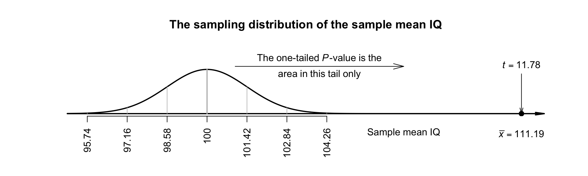
FIGURE 27.8: The sampling distribution for the IQ data. The RQ is one-tailed so the $P$-value is the area in one tail.

We conclude:

Very strong evidence exists in the sample ($t = 11.78$; one-tailed $P < 0.001$) that the population mean IQ in students at Griffith University is greater than $100$ (mean $111.19$; $95$% CI: $109.29$ to $113.09$; $n = 224$).

The test is about the mean IQ; individual students may have IQs less than $100$.

Since the sample size is much larger than $25$, this conclusion is statistically valid. The sample is not a random sample from the population of all GU students (the students are mostly first-year, undergraduate psychological science students). However, these students may be somewhat representative of all GU students. In any case, the results probably apply to first-year, undergraduate psychological science students at GU.

The difference between the general population IQ of $100$ and the sample mean IQ of GU students is only small: about $11$ IQ units (less than one standard deviation). Possibly, this difference has very little practical importance, even though the statistical evidence suggests that the difference cannot be explained by chance.

IQ scores are designed to have a standard deviation of $\sigma = 15$ in the general population. If this applies for university students too (and we do not know if it does), the standard error is $\text{s.e.}(\bar{x}) = \sigma/\sqrt{n} = 15/\sqrt{130} = 1.0022$, and the test-statistic is then a $z$-score: $$z = \frac{\bar{x} - \mu}{\text{s.e.}(\bar{x})} = \frac{111.19 - 100}{1.0022} = 11.87.$$ The conclusions do not change: the $P$-value is still extremely small.

27.10 Chapter summary

These steps are used to test a hypothesis about a population mean $\mu$.

• Write the null hypothesis ($H_0$) and the alternative hypothesis ($H_1$); initially assume the value of $\mu$ in the null hypothesis to be true.
• Describe the sampling distribution, which describes what to expect from the sample mean based on this assumption: under certain statistical validity conditions, the sample mean varies with:
  • an approximate normal distribution,
  • with sampling mean whose value is the value of $\mu$ (from $H_0$), and
  • having a standard deviation of $\displaystyle \text{s.e.}(\bar{x}) =\frac{s}{\sqrt{n}}$.
• Compute the value of the test statistic: $$t = \frac{ \bar{x} - \mu}{\text{s.e.}(\bar{x})},$$ where $\mu$ is the hypothesised value given in the null hypothesis.
• The $t$-value is like a $z$-score, and so an approximate $P$-value can be estimated using the $68$--$95$--$99.7$ rule or tables, or found using software. Use the $P$-value to make a decision, and write a conclusion.
• Check the statistical validity conditions.

The following short video may help explain some of these concepts:

27.11 Quick review questions

The usual recommendation for a safe gap between travelling vehicles in traffic (a 'headway') is at least $1.9\,\text{s}$ (often rounded to $2\,\text{s}$ for the public). Majeed et al. (2014) studied $n = 28$ streams of traffic in Birmingham, Alabama found the mean headway was $1.1915\,\text{s}$, with a standard deviation of $0.231\,\text{s}$. The researchers wanted to test if the mean headway in Birmingham was less than the recommended $1.9\,\text{s}$.

Are the following statements true or false?

1. The standard error of the mean is $0.231\,\text{s}$. TRUE FALSE
2. The null hypothesis is 'The sample mean headway is $1.9\,\text{s}$'. TRUE FALSE
3. The alternative hypothesis 'The population mean is less than $1.9\,\text{s}$'. TRUE FALSE
4. The test is one-tailed. TRUE FALSE
5. The value of the test statistic is $t = -16.23$. TRUE FALSE
6. The one-tailed $P$-value is very small. TRUE FALSE
7. There is no evidence to support the alternative hypothesis. TRUE FALSE

0 of 7 correct

27.12 Exercises

Answers to odd-numbered exercises are given at the end of the book.

Exercise 27.1 Azwari and Hamsa (2021) studied driving speeds in Malaysia, and recorded the speeds of vehicles on various roads. One RQ was whether the mean speed of cars on one particular road was the posted speed limit of $90\,\text{km}.\text{h}^{-1}$, or whether it was higher.

The researchers recorded the speed of $n = 400$ vehicles on this road, and found the mean and standard deviation of the speeds of individual vehicles were $\bar{x} = 96.56$ and $s = 13.874\,\text{km}.\text{h}^{-1}$.

1. Define the parameter of interest.
2. Write the statistical hypotheses.
3. Compute the standard error of the sample mean.
4. Sketch the sampling distribution of the sample mean for $n = 400$.
5. Compute the test statistic, a $t$-score.
6. Determine the $P$-value, and write a conclusion.
7. Is the test statistically valid?

Exercise 27.2 A competitive slalom competitor completed $n = 30$ attempts on a $38.8\,\text{m}$ kayak slalom course to assess the accuracy of a GPS tracking system (Macdermid, Coppelmans, and Cochrane 2022). The trials produced a mean distance, recorded by the GPS, as $36.54\,\text{m}$ with a standard deviation of $2.07\,\text{m}$.

1. Define the parameter of interest.
2. Write the statistical hypotheses.
3. Compute the standard error of the sample mean.
4. Sketch the sampling distribution of the sample mean for $n = 30$.
5. Compute the test statistic, a $t$-score.
6. Determine the $P$-value, and write a conclusion.
7. Is the test statistically valid?

Exercise 27.3 Greenlee, DeLucia, and Newton (2018) conducted a study of human--automation interaction with automated vehicles. They were interested in whether the average mental demand of 'drivers' of automated vehicles was higher than the average mental demand for ordinary tasks.

In the study, the $n = 22$ participants 'drove' (in a simulator) an automated vehicle for $40\,\text{mins}$. While driving, the drivers monitored the road for hazards. The researchers assessed the 'mental demand' placed on these drivers, where scores over $50$ 'typically indicate substantial levels of workload' (p. 471). For the sample, the mean score was $84.00$ with a standard deviation of $22.05$.

Is there evidence of a 'substantial workload' associated with monitoring roadways while 'driving' automated vehicles?

Exercise 27.4 Health departments recommend that hot water be stored at $60$^oC or higher, to kill legionella bacteria (for example, Health and Safety Executive, UK). Alary and Joly (1991) studied $n = 178$ Quebec homes with electric water heaters to see if the mean water temperature was less than $60$^oC (i.e., at risk).

The mean temperature was $56.6$^oC, with a standard error of $0.4$^oC. Is there evidence the mean water temperature in Quebec is too low to kill legionella bacteria?

Exercise 27.5 [Dataset: CherryRipe] A Cherry Ripe is a popular Australian chocolate bar. In 2017, 2018 and 2019, I sampled some Cherry Ripe Fun Size bars. The packaging claimed that the Fun Size bars weigh $14\,\text{g}$ (on average).

1. Use the software output (Fig. 27.9) to determine if the mean weight is $14\,\text{g}$ or not.
2. Explain the difference in the meaning of SD and SE in this context.

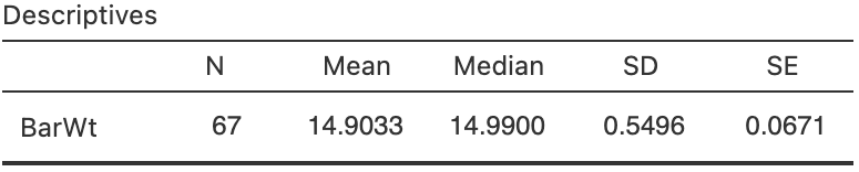
FIGURE 27.9: Software output for the Cherry Ripes data.

Exercise 27.6 (This study was also seen in Exercise 23.6.) B. Williams and Boyle (2007) asked $n = 199$ paramedics to estimate the amount of blood on four different surfaces. When the actual amount of blood spilt on concrete was $\,1000\,\text{mL}$, the mean guess was $846.4\,\text{mL}$ (with $s = 651.1\,\text{mL}$).

Is there evidence that the mean guess is $1\,000\,\text{mL}$ (the true amount)? Is this test statistically valid?

Exercise 27.7 Lin et al. (2021) compared the average sleep times of Taiwanese pre-school children to the recommendation (of at least $10\,\text{h}$ per night). Using the summary of the data for weekend sleep-times (Table 27.1), do girls get less than $10\,\text{h}$ of sleep per night, on average? Do boys?

TABLE 27.1: Summary information for the Taiwanese pre-schoolers sleep times (in h).

	Sample size	Sample mean	Sample std dev.
Boys	$47$	$8.50$	$0.48$
Girls	$39$	$8.64$	$0.37$

Exercise 27.8 [Dataset: LHconc] Feng, Huang, and Ma (2017) assessed the accuracy of two instruments from a clinical laboratory, by comparing the reported luteotropichormone (LH) concentrations to known, pre-determined values using $n = 36$ samples. Use hypothesis tests to determine how the instruments perform, for both high- and mid-level LH concentrations (using the information in below an in Table @(tab:QualityControlDataSummary)).

Show 102550100 entries

The quality-control data: LH levels (in mIU/mL) for two instruments.

	High level	Mid level	High level	Mid level
1	61.63	18.36	62.64	19.12
2	63.11	18.77	64.36	19.07
3	66.88	18.98	66.06	19.58
4	62.56	17.97	65.39	19.35
5	66.12	19.69	66.85	19.65
6	65.34	19.63	65.56	19.13
7	64.83	19.5	66.6	19.55
8	64.22	19.39	66.9	19.85
9	65.54	19.87	65.5	19.45
10	65.33	19.66	65.92	19.87

Showing 1 to 10 of 36 entries

Previous1234Next

TABLE 27.2: Summary of the quality-control data for LH levels (in mIU/mL) for two instruments.

	High level	Mid level	High level	Mid level
Mean of data	$64.310$	$19.240$	$64.970$	$19.400$
Std dev. of data	$\phantom{0}1.700$	$\phantom{0}0.588$	$\phantom{0}1.029$	$\phantom{0}0.413$
Pre-determined target	$64.220$	$19.010$	$65.050$	$19.450$

Exercise 27.9 [Dataset: PizzaSize] (This study was also seen in Exercise 23.10.) In 2011, Eagle Boys Pizza ran a campaign that claimed that Eagle Boys pizzas were 'Real size $12$-inch large pizzas' (P. K. Dunn 2012). Eagle Boys made the data from the campaign publicly available. Using the summary of the diameters of a sample of $125$ of their large pizzas (Fig. 27.10), test the company's claim:

For Eagle Boys' pizzas, is mean diameter actually $12$ inches, or not?

1. What is the parameter of interest?
2. Write down the values of $\bar{x}$ and $s$.
3. Determine the value of the standard error of the mean.
4. Write the hypotheses to test if the mean pizza diameter is $12$ inches.
5. Is the alternative hypothesis one- or two-tailed? Why?
6. Draw the normal distribution that shows how the sample mean pizza diameter would vary by chance, even if the population mean diameter was $12$ inches.
7. Compute the $t$-score for testing the hypotheses.
8. What is the approximate $P$-value using the $68$--$95$--$99.7$ rule?
9. Write a conclusion: do pizzas have a mean diameter of $12$ inches, as claimed?
10. Is it reasonable to assume the statistical validity conditions are satisfied?

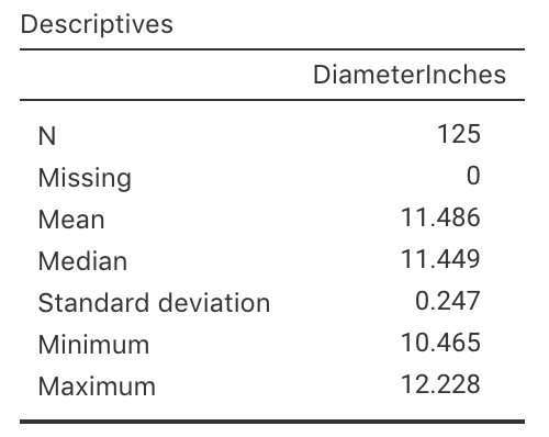
FIGURE 27.10: Summary statistics for the diameter of Eagle Boys large pizzas.

Exercise 27.10 Saxvig et al. (2021) studied the length of sleep each night for a 'large and representative sample of Norwegian adolescents' (p. 1) aged $16$ and $17$ years of age. The recommendation is for adolescents to have at least $8\,\text{h}$ of sleep each night.

In the sample of $n = 3\,972$ individuals, the mean amount of sleep on schools days was $6\,\text{h}$ $43\,\text{mins}$ (i.e., $403\,\text{mins}$), with a standard deviation of $87\,\text{mins}$. On non-school days, the mean amount of sleep was $8\,\text{h}$ $38\,\text{mins}$ (i.e., $518\,\text{mins}$), with a standard deviation of $98\,\text{mins}$.

Do Norwegian adolescents appear to meet the guidelines of having 'at least $8\,\text{h}$' sleep each night on school days? On non-school days?

---

Peter K. Dunn, 2024: CC BY-NC-SA 4.0