20 Models and normal distributions

So far, you have learnt to ask an RQ, design a study, describe and summarise the data, and understand sampling variation. In this chapter, you will learn to:

• describe and draw normal distributions.
• use $z$-scores to compute probabilities related to normal distributions.
• work 'backwards' from probabilities for normal distributions.

20.1 Introduction

As seen in Chap. 19, many different samples could be drawn from a population, and the value of the statistic varies from sample to sample. The challenge of research is that only one of these countless possible samples is observed. The distribution of possible values of the statistic that could be observed from all possible samples is a sampling distribution.

Remember: studying a sample leads to the following observations:

• every sample is likely to be different.
• we observe just one of the many possible samples.
• every sample is likely to yield a different value for the statistic.
• we observe just one of the many possible values for the statistic.

Since many values for the statistic are possible, the possible values of the statistic vary (called sampling variation) and have a distribution (called a sampling distribution).

As seen in Chap. 19, sampling distributions often have a normal distribution (or bell-shaped distribution). That is, the normal distribution is often used to describe the sampling distribution. We now study normal distributions, as they appear in many places in research.

20.2 Normal distributions: examples

In Chap. 19, we saw that the proportion of odd spins in $15$ spins of a roulette wheel could vary; similarly, the mean spin from $15$ spins could vary (Fig. 20.1). In both cases, these sampling distributions had a rough normal distribution shape. This is true for larger numbers of spins also (Figs. 19.1 and 19.2).

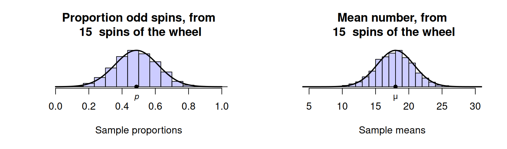
FIGURE 20.1: Sampling distributions for the proportion of odd spins (left), and the mean of the numbers after $15$ roulette wheel spins (right) are approximate normal distributions. The solid lines are theoretical normal distributions.

The histograms in Fig. 20.1 are based on results from a limited number of simulations. The solid lines shown in Fig. 20.1 are actual normal distributions, and represent how the histogram might appear theoretically if we used an infinite number of simulations. The normal distributions are models for what might occur in the population, so normal distributions are also called normal models. Since the models represent populations, the mean of the model is denoted $\mu$ and the standard deviation is denoted $\sigma$.

A model is a theoretical or ideal concept. A model skeleton isn't $100$% accurate and certainly not exactly like your skeleton; nonetheless, it suitably approximates reality. None of us probably have a skeleton exactly like the model, but the model is still useful and helpful. Likewise, a sampling distribution may not have exactly a normal shape, but the model is still useful and helpful. The model is a way of describing a theoretical distribution in the population. A model is a simple (but not overly simple) approximation to reality.

The histograms in Fig. 20.1 are not exactly normal distributions, but are very close to normal distributions, and certainly close enough for most purposes. Many, but not all, sampling distributions have approximate normal distributions.

Sampling distributions represent theoretical distributions of sample statistics, not the distribution of sample data. When the sampling distribution is a normal distribution, the mean of the distribution is called the sampling mean and the standard deviation is called the standard error.

Apart from their use in modelling theoretical sampling distributions, some quantitative variables have approximate normal distributions too, when the distribution of the data in the population can be approximately modelled by a normal distribution.

Example 20.1 (Normal distributions of data) Some quantitative variables have approximate normal distributions. Figure 20.2 (left panel) shows the diastolic blood pressure of $398$ Americans (Willems et al. 1997; Schorling et al. 1997). Figure 20.2 (right panel) shows the weight of $83$ male Leadbeater's possums (J. L. Williams et al. 2022).

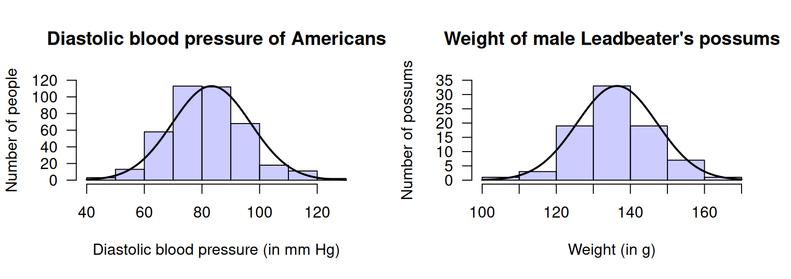
FIGURE 20.2: Two normal distributions. Left: diastolic blood pressure of a sample of $398$ Americans. Right: the weight of a sample of $83$ male Leadbeater's possums. The solid lines are the approximate normal model for the variable in the population.

20.3 Normal distributions and the 68--95--99.7 rule

Normal distributions have a shape that is symmetric about the mean, with a bell shape. Half the values are greater than the mean, and half the values are less than the mean. The total probability represented by a normal distribution is one (or $100$%). For example, every sample will produce a sample proportion between $0$ and $1$ and so is represented somewhere in Fig. 20.1 (left panel); every American has a diastolic blood pressure and so is represented somewhere in Fig. 20.2 (left panel); every male Leadbeater's possum has a weight and so is represented somewhere in Fig. 20.2 (right panel).

In theory, no upper limit or lower limit exists for a variable modelled using a normal distribution. In practice, this is rarely true, but usually never presents a problem. Consider the normal distributions in Fig. 20.2, for example. The normal distribution shown for the diastolic blood pressure (left panel) has no lower or upper limit in theory, but all practical values of diastolic blood pressure are captured by that part of the normal distribution shown. The normal distribution implies almost no-one has a diastolic blood pressure below $40\,\text{mm}$ Hg or above $130\,\text{mm}$ Hg.

One of the most important properties of normal distributions is the 68--95--99.7 rule (sometimes called the empirical rule).

Definition 20.1 (The 68--95--99.7 rule) For any quantity modelled by a normal distribution:

• approximately $68$% of values lie within $1$ standard deviation of the mean.
• approximately $95$% of values lie within $2$ standard deviations of the mean.
• approximately $99.7$% of values lie within $3$ standard deviations of the mean.

These properties are true for all normal distributions, whatever the quantity, whatever the value of the mean, and whatever the value of the standard deviation (Fig. 20.3).

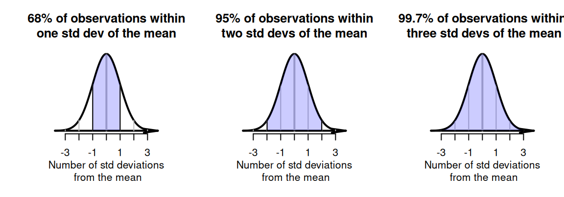
FIGURE 20.3: The $68$--$95$--$99.7$ rule. The shaded regions correspond to the central $68$%, $95$% and $99.7$%.

Example 20.2 (Heights of females) Suppose the heights of Australian adult females in the population can be modelled with a normal distribution having a mean of $\mu = 162\,\text{cm}$, and a standard deviation of $\sigma = 7\,\text{cm}$, and follow a normal distribution (Fig. 20.4). Using the $68$--$95$--$99.7$ rule, approximately $68$% of Australian women will be between $162 - 7 = 155\,\text{cm}$ and $162 + 7 = 169\,\text{cm}$ tall using this model. Similarly, approximately $95$% of Australian women will be between $162 - (2\times 7) = 148\,\text{cm}$ and $162 + (2\times 7) = 176\,\text{cm}$ tall.

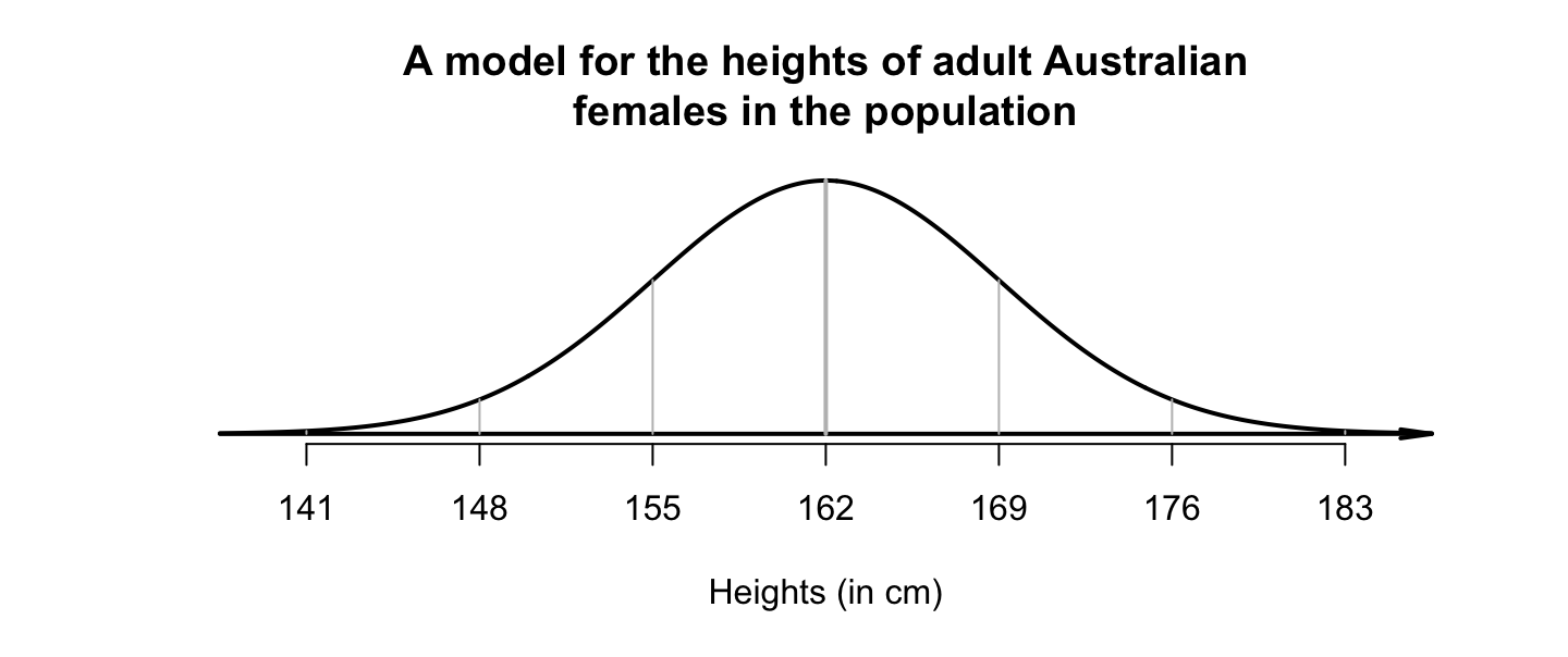
FIGURE 20.4: A model for the height of adult Australian females in the population.

These regions under the normal curve are probabilities, are often called areas, and are sometimes expressed as percentages.

20.4 Standardising ($z$-scores)

Since the $68$--$95$--$99.7$ rule (Def. 20.1) applies for all normal distributions, the percentages in the rule only depend on how many standard deviations ($\sigma$) a value ($x$) is from the mean ($\mu$). This information can be used to learn more about how values are distributed in a normal distribution.

For example, suppose heights of Australian adult females can be modelled with a normal distribution having a mean of $\mu = 162\,\text{cm}$, and a standard deviation of $\sigma = 7\,\text{cm}$ (Example 20.2). Using this model, the proportion of Australian adult women taller than $169\,\text{cm}$ can be determined.

From a picture (Fig. 20.5, left panel), $162 + 7 = 169\,\text{cm}$ is one standard deviation above the mean. Since $68$% of values are within one standard deviation of the mean, $32$% are outside that range (some shorter; some taller). Hence, $16$% are taller than one standard deviation above the mean, so the answer is about $16$%. (Another $16$% are shorter than one standard deviation below the mean, or less than $162 - 7 = 155\,\text{cm}$ in height.)

Again, the percentages only depend on how many standard deviations ($\sigma$) the value ($x$) is from the mean ($\mu$), and not the actual values of $\mu$ and $\sigma$.

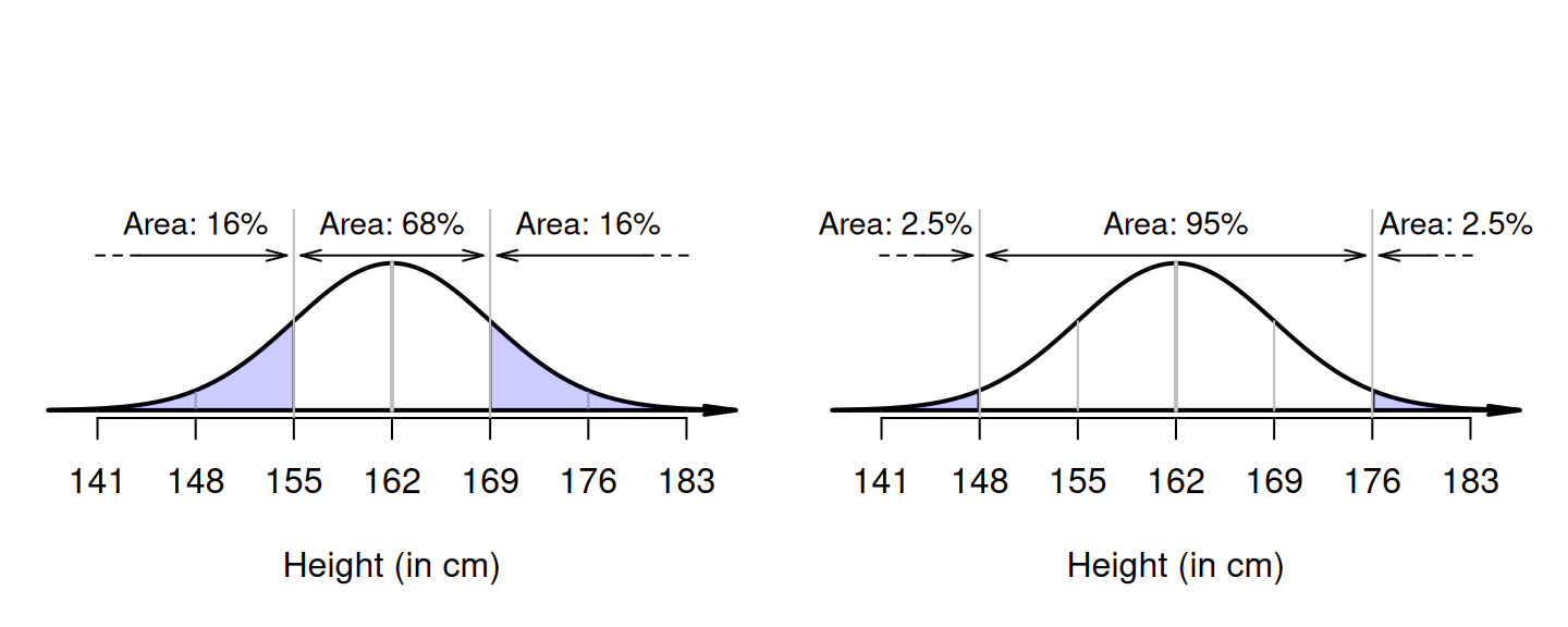
FIGURE 20.5: Left: what proportion of Australian adult females are taller than $169\,\text{cm}$? Right: what proportion of Australian adult females are shorter than $148$?

Example 20.3 (The 68-95-99.7 rule) Consider again the heights of Australian adult females. Using this model, what proportion are shorter than $148\,\text{cm}$?

Again, drawing a picture is helpful (Fig. 20.5, right panel). Since $162 - (2\times 7) = 148$, $148\,\text{cm}$ is two standard deviations below the mean. Since $95$% of values are within two standard deviation of the mean, $5$% are outside that range (half smaller, half larger; see Fig. 20.5, right panel), so that $2.5$% are shorter than $148\,\text{cm}$. (Another $2.5$% are taller than $162 + 14 = 176\,\text{cm}$.)

Again, the percentages only depend on how many standard deviations ($\sigma$) the value ($x$) is from the mean ($\mu$). The number of standard deviations that an observation is from the mean is called a $z$-score. A $z$-score is computed using $$z = \frac{ x - \mu}{\sigma},$$ where $\sigma$ is the standard deviation quantifying the variation in the $x$-values. Converting values to $z$-scores is called standardising.

Definition 20.2 (z-score) A $z$-score measures how many standard deviations a value $x$ is from the mean. In symbols: $$\begin{equation} z = \frac{x - \mu}{\sigma}, \tag{20.1} \end{equation}$$ where $\mu$ is the mean of the distribution, and $\sigma$ is the standard deviation of the distribution (measuring the variation in the $x$-values).

The $z$-score is also called the standardised value or standard score. Note that:

• $z$-scores are negative for observations below the mean.
• $z$-scores are positive for observations above the mean.
• $z$-scores have no units (that is, not measured in kg, or cm, etc.).

Example 20.4 (z-scores) Consider the model for the heights of Australian adult females again. From earlier, the $z$-score for a height of $169\,\text{cm}$ is $$z = \frac{x-\mu}{\sigma} = \frac{169 - 162}{7} = 1,$$ one standard deviation above the mean. Similarly, the $z$-score for a height of $148\,\text{cm}$ is $$z = \frac{x-\mu}{\sigma} = \frac{148 - 162}{7} = -2,$$ two standard deviations below the mean.

Example 20.5 (The 68-95-99.7 rule) Consider the model for the heights of Australian adult females: a normal distribution, mean $\mu = 162\,\text{cm}$, standard deviation $\sigma = 7\,\text{cm}$ (Fig. 20.6). Using this model:

• a height of $162\,\text{cm}$ is zero standard deviations from the mean: $z = 0$.
• $155\,\text{cm}$ is one standard deviation below the mean: $z = -1$.
• $169\,\text{cm}$ is one standard deviation above the mean: $z = 1$.
• $148\,\text{cm}$ and $176\,\text{cm}$ correspond to $z = -2$ and $z = 2$ respectively.
• $141\,\text{cm}$ and $183\,\text{cm}$ correspond to $z = -3$ and $z = 3$ respectively.

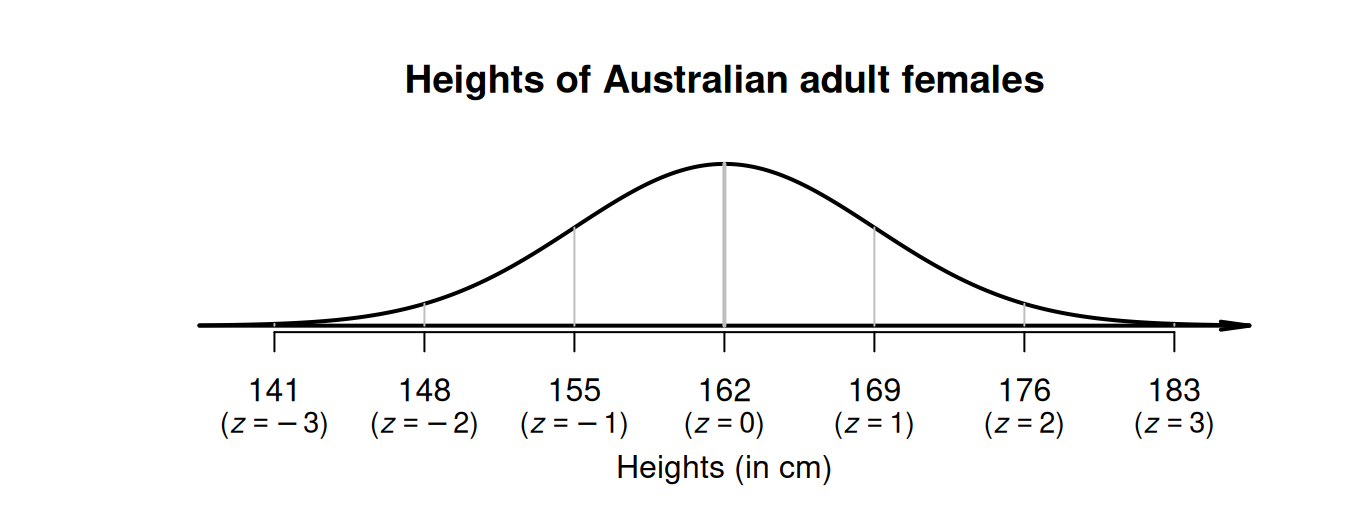
FIGURE 20.6: The $68$--$95$--$99.7$ rule and the heights of Australian adult females.

20.5 Approximating areas (percentages) using the $68$--$95$--$99.7$ rule

As seen above, the $68$--$95$--$99.7$ rule can be used to approximate percentages under normal distributions. The rule can even be used for values that do not exactly align with $1$, $2$ or $3$ standard deviations from the mean.

Suppose again that heights of Australian adult females can be modelled with a normal distribution with a mean of $\mu = 162\,\text{cm}$, and a standard deviation of $\sigma = 7\,\text{cm}$ (Fig. 20.6). To find the proportion of women shorter than $145\,\text{cm}$, first draw the situation (Fig. 20.7). Proceeding as before, we ask 'How many standard deviations from the mean is $145\,\text{cm}$?' Using Equation (20.1), $145\,\text{cm}$ corresponds to a $z$-score of $$\begin{equation} z = \frac{145 - 162}{7} = -2.4285... \tag{20.2} \end{equation}$$ which is about $2.43$ standard deviations below the mean.

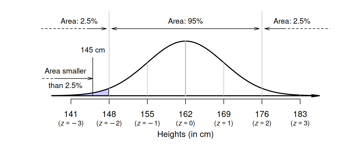
FIGURE 20.7: What proportion of Australian adult females are shorter than $145\,\text{cm}$?

What percentage of observations are less than this $z$-score? This case is not covered by the $68$--$95$--$99.7$ rule, though the rule can be used to make rough estimates.

About $2.5$% of observations are less than $2$ standard deviations below the mean; that is, about $2.5$% of women are shorter than $148\,\text{cm}$. So the percentage of females shorter than $145$(that is, even shorter than $148\,\text{cm}$, and so further into the tail of the distribution) will be smaller than $2.5$%. While we don't know the probability exactly, it will be smaller than $2.5$%.

Percentages found this way are very approximate, but often sufficient. However, more accurate percentages are found using tables compiled for this very purpose (Appendix B.1). We now learn to use these tables.

20.6 Exact areas (percentages) using tables

Areas under normal distributions can be found using online tables, or hard copy tables., for any $z$-score. The online tables are easier to use, but only the online tables are explained in this online book (see the hard-copy version for the hard-copy tables, and instruction for using use the hard-copy tables). The tables (Appendix B.1) work with $z$-scores to two decimal places, so consider the $z$-score from Sect. 20.5 as $z = -2.43$.

The online tables can be found in Appendix B.1. In the tables, enter the $z$-score in the the box z.score: then, the probability of finding a $z$-score less than (i.e., to the left of) this value is shown. The tables give the area as $0.0075$.

The tables always give the area to the left of the $z$-score that is looked up.

Our tables always give the area to the left of the $z$-score.

Either the hard-copy or online tables gives an answer of $0.75$%. This is consistent with the rough answer using the $68$--$95$--$99.7$ rule: a value less than $2.5$%.

20.7 Examples using $z$-scores

The general approach to computing probabilities from normal distributions is:

• draw a diagram, and mark on the value(s) of interest.
• shade the required region of interest.
• compute the $z$-score(s) using Equation (20.1).
• use the tables in Appendix B.1 to compute corresponding areas (percentages).
• deduce the answer.

This approach can be used to answer more complicated questions involving normal distributions.

Example 20.6 (Normal distributions) Mechanised forest harvesting systems were simulated by Aedo-Ortiz, Olsen, and Kellogg (1997), and the diameters of a specific type of tree were modelled using:

• a normal distribution, with
• a mean of $\mu = 8.8$ inches, and
• a standard deviation of $\sigma = 2.7$ inches.

Using this model, what is the probability that a randomly-chosen tree has a diameter greater than $5$ inches?

Following the steps identified earlier:

• draw the appropriate normal curve, and mark on $5$ inches (Fig. 20.8, left panel).
• shade the region 'greater than $5$ inches' (Fig. 20.8, centre panel).
• compute the $z$-score using Equation (20.1): $\displaystyle z = (5 - 8.8)/2.7 = -1.41$ to two decimal places.
• use tables: the probability of a tree diameter shorter than $5$ inches is $0.0793$. (Remember: the tables always give area less than the value of $z$.)
• deduce the answer (Fig. 20.8, right panel): since the total area under the normal distribution is one (or $100$%), the probability of a tree diameter greater than $5$ inches is $1 - 0.0793 = 0.9207$, or about $92$%.

A randomly-chosen tree has a probability of $92$% of having a diameter greater than $5$ inches.

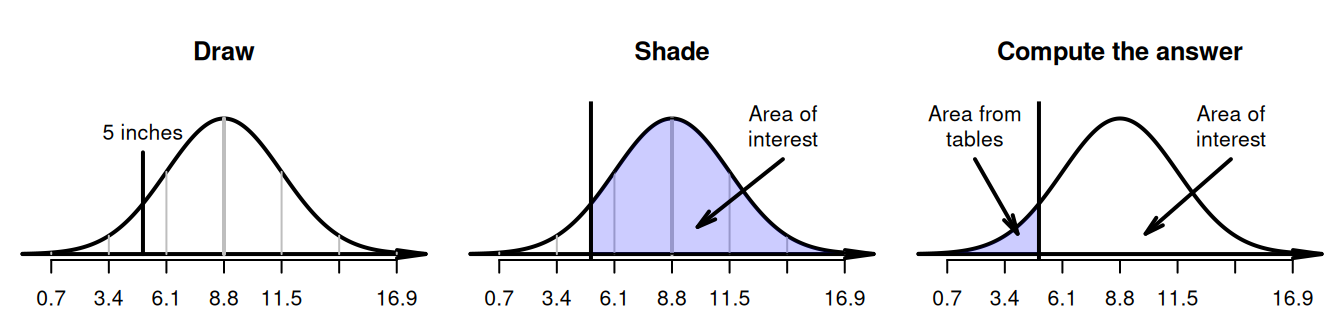
FIGURE 20.8: What proportion of tree diameters are greater than $5$ inches?

Our normal-distribution tables always provide area to the left of the $z$-score. Drawing a picture of the situation is important: it helps visualise getting the area requested from the area the tables provide. Remember: the total area under the normal distribution is one (or $100$%).

Example 20.7 (Normal distributions) These scenarios can be displayed on a diagram as shown in Fig. 20.9 (recall $\mu = 8.8$ inches).

1. Tree diameters between $3$ and $5$ inches: Diagram A.
2. Tree diameters greater than $11$ inches: Diagram B.
3. Tree diameters between $5$ and $11$ inches: Diagram C.
4. Tree diameters less than $11$ inches: Diagram D.

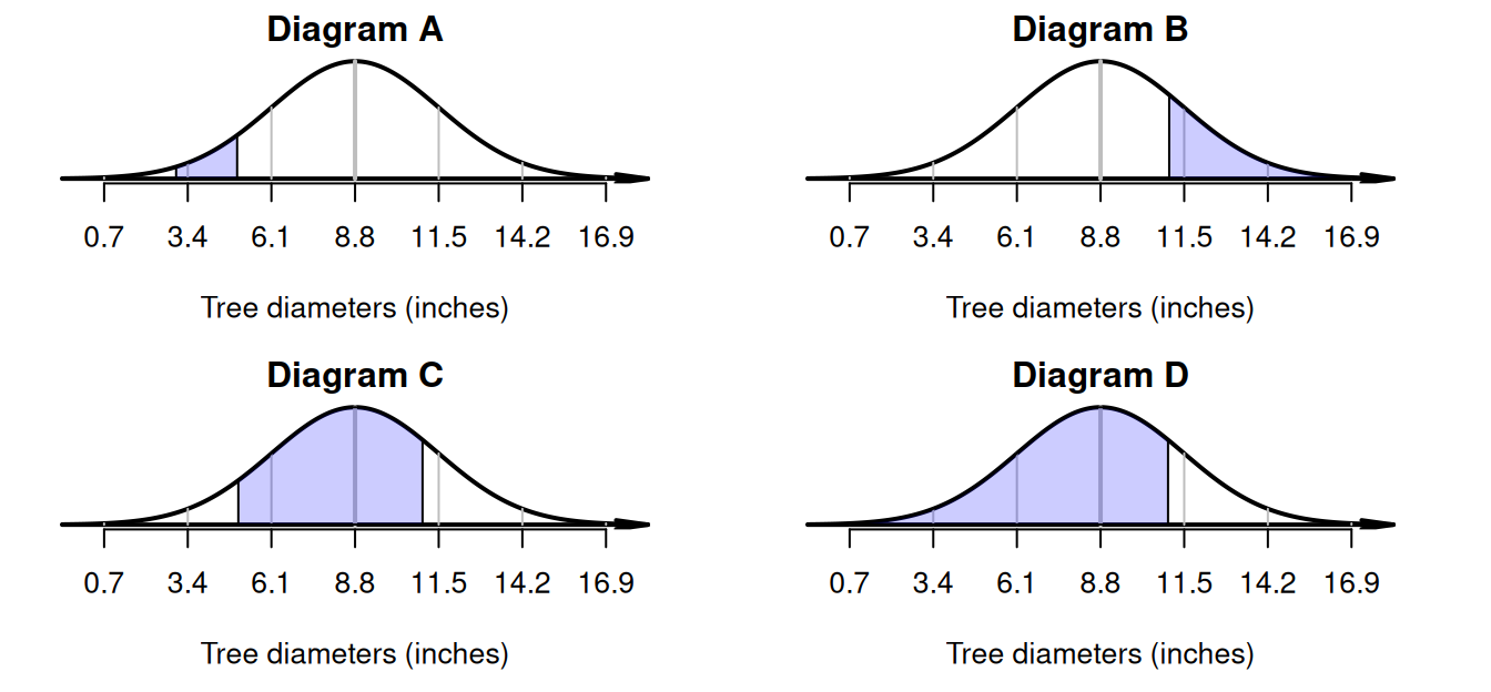
FIGURE 20.9: Scenarios with their corresponding diagrams.

Example 20.8 (Normal distributions) Using the model for tree diameters in Example 20.6, what is the probability that a tree has a diameter between $5$ and $11$ inches?

First, draw the situation, and shade 'between $5$ and $10$ inches' (Fig. 20.9, Diagram C). Then, compute the $z$-scores for both tree diameters:

• $\quad z = (5 - 8.8)/2.7 = -1.41$ (i.e., below the mean).
• $\quad z = (11 - 8.8)/2.7 = 0.81$ (i.e., above the mean).

The tables in Appendix B.1 can then be used to find the area to the left of $z = -1.41$ (which is $0.0793$), and also to find the area to the left of $z = 0.81$ (which is $0.791$). However, neither of these provide the area between $z = -1.41$ and $z = 0.81$.

Looking carefully at the areas from the tables and the area sought, the required area is the area between the two $z$-scores (Fig. 20.10): $0.7910 - 0.0793 = 0.7117$ (see the animation below). The probability that a tree has a diameter between $5$ and $11$ inches is about $0.7117$, or about $71$%.

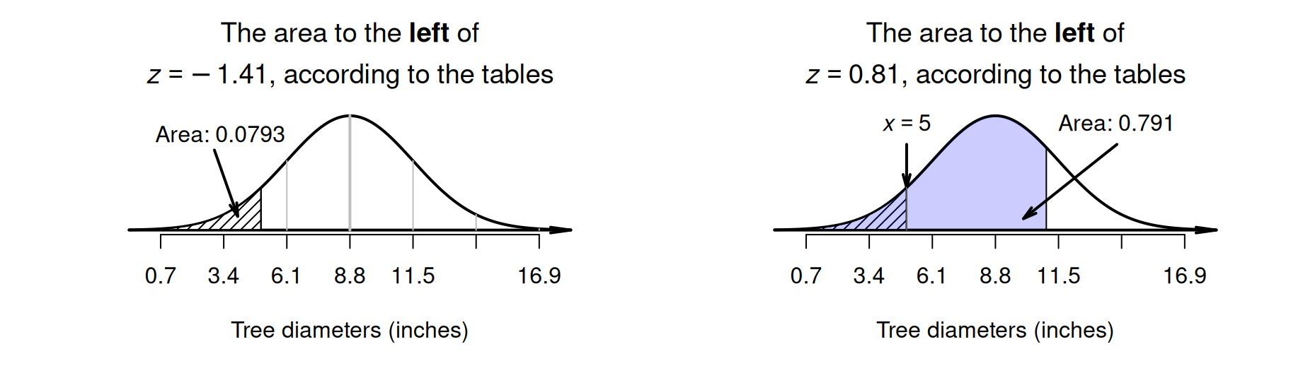
FIGURE 20.10: What proportion of tree diameters are between $5$ and $11$ inches? Left: the hatched area is the area to the left of $z = -1.41$. Right: the shaded area is the area to the left of $z = 0.81$. Neither give us the area we seek directly.

20.8 Unstandardising: working backwards

Using the model for tree diameters in Example 20.6 again, different types of questions can be asked too. Suppose we needed to identify the diameters of the smallest $3$% of trees.

This is a different type of problem than before; previously, the tree diameter was known, so a $z$-score could be computed, and hence a probability (Fig. 20.11). However, here the probability is known, and a tree diameter is sought. That is, working 'backwards' is necessary (Fig. 20.11), so the $z$-tables need to be used 'backwards' too.

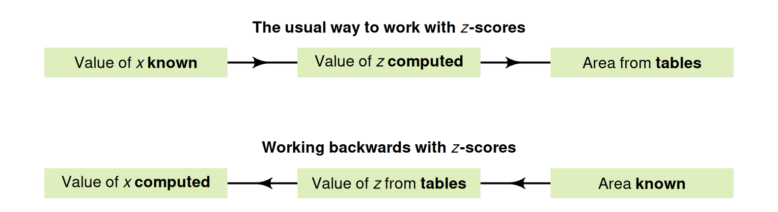
FIGURE 20.11: Working with $z$-scores. In the tables, the areas (probabilities) are in the body of the table, and the $z$-scores are in the margins of the table.

Drawing a rough diagram of the situation again is very helpful (Fig. 20.12). We can only mark the approximate location of the required score, but this is sufficient. Then, tables must be used to determine the corresponding $z$-score. Since the required value will be smaller than the mean, the $z$-score will be negative (to the left of the mean).

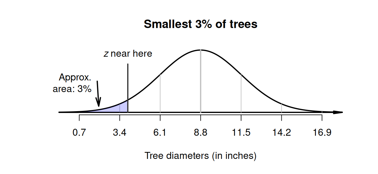
FIGURE 20.12: Tree diameters: the smallest $3$% is shaded. The approximate location of the required $z$-score is drawn.

As before (Sect. 20.6), online tables or hard copy tables can be used (and again the online tables are easier to use). Only the online tables are explained in this online book (see the hard-copy version for the hard-copy tables, and instructions for their use).

The online tables are found in Appendix B.1. In the tables, enter the area to the left of the required unknown value in the box Area.to.left: the $z$-score with this probability to the left is shown.

Using online tables, $z$-score of $z = -1.881$. (The hard-copy tables are less precise, and give $z = -1.88$.)

Our tables always give the area to the left of the $z$-score.

Using either the hard-copy or online tables, the appropriate $z$-value is about $-1.88$ standard deviations below the mean; that is, $z = -1.88$ (Fig. 20.12). The $z$-score can be converted to an observation value $x$ using the unstandardising formula:³ $$x = \mu + z\sigma.$$ Using this unstandardising formula: $$\begin{align*} x &= \mu + (z\times\sigma) \\ &= 8.8 + (-1.88 \times 2.7) = 3.724; \end{align*}$$ that is, about $3$% of trees have diameters less than about $3.72$ inches.

Definition 20.3 (Unstandardising formula) When the $z$-score is known, the corresponding value of the observation $x$ is $$\begin{equation} x = \mu + z\sigma. \tag{20.3} \end{equation}$$ This is called the unstandardising formula.

Example 20.9 (Normal distributions backwards) Using the model for tree diameters in Example 20.6 again, suppose now the diameters of the largest $25$% of trees needs to be identified.

The situation can be drawn (Fig. 20.13). Since an area is given, we need to work 'backwards', so the $z$-tables need to be used 'backwards' too. The largest $25$% implies large trees, so required diameter is larger than the mean (so corresponds to a positive $z$-score).

The tables work with the area to the left of the value of interest, which is $75$% (Fig. 20.13). Using either the hard-copy or online tables, the appropriate $z$-value is $z = 0.674$. Then, the $z$-score can be converted to an observation value $x$ using the unstandardising formula: $$\begin{align*} x &= \mu + (z\times\sigma) \\ &= 8.8 + (0.674 \times 2.7) = 10.621. \end{align*}$$ That is, about $25$% of trees have diameters larger than about $10.6$ inches.

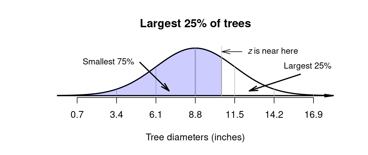
FIGURE 20.13: Tree diameters: the largest $25$% is the same as the smallest $75$%.

20.9 Example: methane production

Huhtanen, Ramin, and Cabezas-Garcia (2016) modelled the retention time of food in sheep, using a normal distribution with the mean retention time as $\mu = 42.5\,\text{h}$, and the standard deviation as $\sigma = 3.68\,\text{h}$. We can draw this normal distribution (Fig. 20.14), and then apply the $68$--$95$--$99.7$ rule:

• about $68$% of retention times are between $38.82$ and $46.18\,\text{h}$.
• about $95$% of retention times are between $35.14$ and $49.86\,\text{h}$.
• about $99.7$% of retention times are between $31.46$ and $53.54\,\text{h}$.

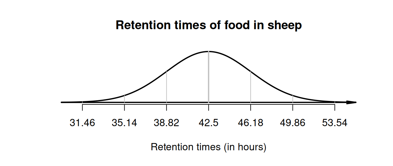
FIGURE 20.14: Retention times of food in sheep.

Example 20.10 (Working with the normal distribution) Using this model, what proportion of sheep have a retention time less than $40\,\text{h}$?

A retention time of $40\,\text{h}$ corresponds to a $z$-score of (Fig. 20.15, top left panel): $$z = \frac{40 - 42.5}{3.68} = -0.68.$$ This is a negative number, since $40\,\text{h}$ is below the mean. Using the tables in Appendix B.1 (that give the area to the left of the $z$-score), the area to the left of $z = -0.68$ is $0.2483$, or about $24.8$%. About $24.8$% of sheep have a retention time less than $40\,\text{h}$.

Example 20.11 (Working with the normal distribution) What proportion of sheep have a retention time greater than $48\,\text{h}$ (two days)?

A retention time of $48\,\text{h}$ corresponds to a $z$-score of $1.49$. Using the normal distribution tables, the area to the left of this $z$-score is $0.9319$, so the area to the right of this $z$-score is $0.0681$ (Fig. 20.15, top right panel).

Example 20.12 (Working with the normal distribution) What proportion of sheep have a retention time between $40$ and $48\,\text{h}$?

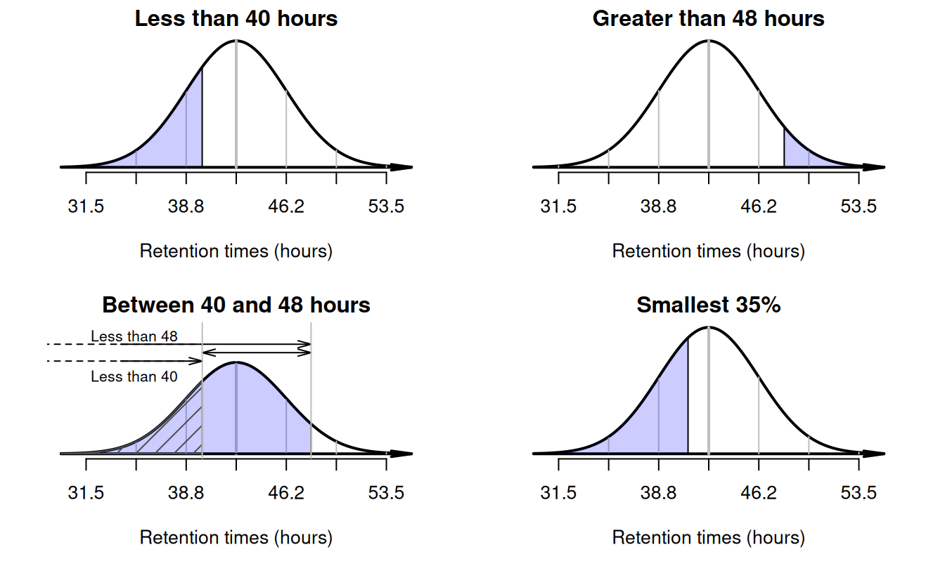
FIGURE 20.15: Plots for retention times in sheep.

A retention time of $40\,\text{h}$ corresponds to $z = -0.68$ and, using the normal distribution tables, the area to the left of $z = -0.68$ is $0.2483$ (Fig. 20.15, bottom left panel; hatched area). But this is not the area that we seek. From earlier, the area to the left of $z = 1.49$ is $0.9319$ (Fig. 20.15, bottom left panel; shaded region). But this is not the area we seek either. From the two areas that we know, we can find the area that we seek (Fig. 20.15, bottom left panel):

• $48\,\text{h}$ corresponds to $z = 1.49$; the area to the left of this $z$-score is $0.9319$.
• $40\,\text{h}$ corresponds to $z = -0.68$; the area to the left of this $z$-score is $0.2483$.
• the difference between these two areas is sought, which is $0.9319 - 0.2483 = 0.6836$.

So the proportion is about $0.684$ (or $68.4$%).

Example 20.13 (Working with the normal distribution) Consider the $35$% of sheep with the shortest retention times. What are these retention times?

The time we seek must be smaller than the mean if it defines the shortest $35$% of retention times. We don't know exactly where to draw the retention time that this corresponds to on the diagram; it's just somewhere to the left of the mean (Fig. 20.15, bottom right panel).

This time, we know the area to the left, but we do not know the value (or $z$-score). This a 'backwards problem', and we need to find the $z$-score 'backwards' (Sect. 20.8). From the hard copy tables, a $z$-score of $z = -0.39$ has an area to the left of $0.3483$, which is as close as we can get. (The online tables are more precise: $z = -0.385$.)

We know the $z$-score, so the retention value is found using the unstandardising formula: $$x = \mu + (z \times \sigma) = 42.5 + (-0.385\times 3.68) = 41.0832.$$ The retention time is about $41.1\,\text{h}$.

20.10 Chapter summary

A model is a way of describing the theoretical distribution of some quantitative quantity. One common model is a normal model or normal distribution, which is a bell-shaped distribution with a theoretical mean $\mu$ and a theoretical standard deviation $\sigma$. Probabilities can be computed from normal distributions using $z$-scores, the $68$--$95$--$99.7$ rule, or tables.

20.11 Quick review questions

Consider again the model for tree diameters in Example 20.6 (Aedo-Ortiz, Olsen, and Kellogg 1997): a normal distribution with $\mu = 8.8$ inches, and $\sigma = 2.7$ inches.

Are the following statements true or false?

1. A tree diameter of $10.2$ inches corresponds to a $z$-score of $(10.2 - 8.8)/2.7 = 0.519$. TRUE FALSE
2. The probability that a tree has a diameter less than $10.2$ inches is about $0.70$. TRUE FALSE
3. The probability that a tree has a diameter greater than $10.2$ inches is about $0.70$. TRUE FALSE
4. A tree diameter of $6$ inches corresponds to a $z$-score of $1.04$. TRUE FALSE
5. The probability that a tree has a diameter less than $6$ inches is $0.15$. TRUE FALSE
6. The probability that a tree has a diameter greater than $6$ inches is $0.85$. TRUE FALSE

0 of 6 correct

20.12 Exercises

Answers to odd-numbered exercises are given at the end of the book.

Exercise 20.1 Are the following statements true or false?

1. The unstandardising formula can be used to compute probabilities. True False
2. About $68$% of observations are within two standard deviations of the mean.
   True False
3. Positive $z$-scores correspond to values larger than the mean.
   True False
4. A $z$-score tells us how many standard deviations a value is away from the mean.
   True False

Exercise 20.2 Are the following statements true or false?

1. A $z$-score larger than $4$ is impossible.
   True False
2. A $z$-score of zero is located at the mean value of the population.
   True False
3. About $5$% of observations are less than two standard deviations below the mean.
   True False
4. A $z$-score of zero means a calculation error has been made.
   True False

Exercise 20.3 Determine the probability that an observation is less than the following $z$-scores.

1. $z = 1.84$.
2. $z = -2.09$.

 

3. $z = -5.34$.
4. $z = 4.25$

Exercise 20.4 Determine the probability that an observation is greater than the following $z$-scores.

1. $z = -0.48$.
2. $z = 1.03$.

 

3. $z = -4.00$.
4. $z = 0.00$

Exercise 20.5 Growth charts released by the World Health Organisation (WHO 2006) showed that girls aged five-years-old with a height of $100\,\text{cm}$ are said to have a $z$-score of $z = –2$. What does this mean?

Exercise 20.6 Growth charts released by the World Health Organisation (WHO 2006) showed that girls aged five-years old with a height of $120\,\text{cm}$ are said to have a $z$-score of $z = +2$. What does this mean?

Exercise 20.7 IQ scores are designed to have a mean of $100$ and a standard deviation of $15$. Match the diagram in Fig. 20.16 with the meaning.

1. IQs greater than $110$.
2. IQs between $90$ and $115$.

 

3. IQs less than $110$.
4. IQs greater than $85$.

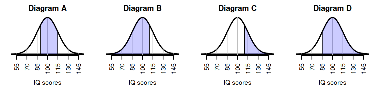
FIGURE 20.16: Match the diagram with the description.

Exercise 20.8 IQ scores are designed to have a mean of $100$ and a standard deviation of $15$. Match the diagram in Fig. 20.17 with the meaning.

1. The largest $25$% of IQ scores.
2. The smallest $10$% of IQ scores.

 

3. The largest $70$% of IQ scores.
4. The smallest $60$% of IQ scores.

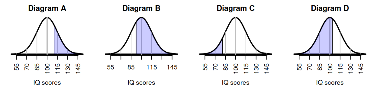
FIGURE 20.17: Match the diagram with the description.

Exercise 20.9 The $68$--$95$--$99.7$ rule states that approximately $68$% of observations are within one standard deviation of the mean. Use the tables in Appendix B.1 to compute a more precise value for the percentage of observations within one standard deviation of the mean. Comment.

Exercise 20.10 The $68$--$95$--$99.7$ rule states that approximately $95$% of observations are within two standard deviations of the mean. Use the tables in Appendix B.1 to compute a more precise value for the percentage of observations within two standard deviations of the mean. Comment.

Exercise 20.11 Consider again the study by Aedo-Ortiz, Olsen, and Kellogg (1997) (Example 20.6), who studied the diameter of trees in certain forests. The tree diameters can be modelled as having a normal distribution, with a mean of $\mu = 8.8$ inches, and a standard deviation of $\sigma = 2.7$ inches. Using this model, answer these questions.

1. What is the probability that a tree will have a diameter less than $8$ inches?
2. What is the probability that a tree will have a diameter greater than $9$ inches?
3. What is the probability that a tree will have a diameter between $7$ and $10$ inches?
4. The largest $15$% of trees have what diameters?
5. The smallest $25$% of trees have what diameters?

Exercise 20.12 Pasha et al. (2016) simulated methods for coating corn seeds (with fertiliser and crop protection chemicals, etc.). The seed diameter was modelled with a normal distribution, with mean $7.5\,\text{mm}$ and standard deviation of $0.225\,\text{mm}$. Using this model, answer these questions.

1. What is the probability that a seed has a diameter of more than $8\,\text{mm}$?
   About 2.22About 1.3%About 98.7%
2. What is the probability that a seed has a diameter less than $7.1\,\text{mm}$?
   
   About 96.3%About 3.8%About -1.78
3. What is the probability that a seed has a diameter between $7.5$ and $8\,\text{mm}$?
   
   About 0.89About 48.7%About 2.22About 50%About 98.7%
4. What is the diameter of the smallest $30$% of seeds?
   
   Smaller than about 7.62mmLarger than about 7.38mmAbout -0.524Smaller than about 7.38mm
5. What is the diameter of the largest $90$% of the seeds?
   
   Less than about 7.79mmLarger than about 7.79mmLess than about 7.21mmLarger than about 7.21mmAbout -1.28

Exercise 20.13 Snowden and Basso (2018) studied factors influencing preterm births. They modelled the gestation length of healthy babies with a normal distribution, having a mean of $40$ weeks, and a standard deviation of $1.64$ weeks. Using this model, answer these questions.

1. What proportion of births are longer than $39$ weeks (that is, nine months)?
2. In Australia, a premature birth is defined as a birth occuring before $37$ weeks. What proportion of births are expected to be premature?
3. According to Health Direct, 'Babies born between $32$ and $37$ weeks may need care in a special care nursery'. What proportion of healthy births would be expected to be born between $32$ and $37$ weeks gestation?
4. How long is the gestation length for the longest $5$% of pregnancies?
5. How long is the gestation length for the shortest $10$% of pregnancies?

Exercise 20.14 A new method for evaluating bridge loads (O’Brien et al. 2018) used a simulation to compare the new method to an existing method. For the simulation, they modelled the gross vehicle mass (GVM) of trucks as having a normal distribution, with a mean of $13$ tonnes and a standard deviation of $1.3$ tonnes.

The Isuzu F-Series trucks in 2025 were rated as having a GVM between $10.7$ and $26.0$ tonnes (depending on the configuration).

1. What is the $z$-score for the lower limit of $10.7$ tonnes?
2. What is the $z$-score for the upper limit of $26.0$ tonnes?
3. What does a negative $z$-score mean in this context?

Exercise 20.15 IQ scores are designed to have a mean of $100$ and a standard deviation of $15$. Mensa is a society for people with a high IQ; specifically, for people who have 'attained a score within the upper two percent of the general population' (Mensa webpage: https://www.mensa.org/). What IQ score is needed to join Mensa?

Exercise 20.16 IQ scores are designed to have a mean of $100$ and a standard deviation of $15$. Zagorsky (2016) reports that the US Military must 'reject all military recruits whose IQ is in the bottom $10$% of the population' (Zagorsky (2016), p. 403). What IQs scores lead to a rejection from the US military?

Exercise 20.17 A study of the impact of charging electric vehicles (EVs) on electricity demands (Affonso and Kezunovic 2018) modelled the time at which people began charging their EVs at home. Based on a survey (US Department of Transportation 2011), they modelled the time at which EVs began charging as having a mean of $5$:$30$pm, with a standard deviation of $2.28\,\text{h}$. For this model:

1. What is the probability that an EV will begin charging after $9$pm?
2. What is the probability that an EV will begin charging before $5$pm?
3. What is the probability that an EV will begin charging between $5$pm and $6$pm?
4. $30$% of the EVs begin charging after what time?
5. The earliest $15$% of charging begins when?

Hint: this question is easier if you convert times into 'minutes after $5$:$30$'.

---

Peter K. Dunn, 2024: CC BY-NC-SA 4.0