25 Making decisions

So far, you have learnt to ask an RQ, design a study, describe and summarise the data, and form confidence intervals. In this chapter, you will learn how decisions are made in science, so you can answer RQs. You will learn to:

state the two broad reasons that might explain the difference between the values of the statistic and parameter.
explain how decisions are made in research.

25.1 Introduction: drawing cards

Suppose I produce a pack of cards, and shuffle them well. The event of interest is 'the number of red cards when I draw $25$ cards from the pack, with replacement'. ('With replacement' means that, after drawing a card, I place the card back into the pack, and reshuffle before drawing a new card; each draw is then from an identical, complete pack of $52$ cards.) The pack of cards can be considered the population. In a standard pack, the proportion of red cards is $p = 0.5$ for each draw, because sampling is with replacement. $\hat{p}$ is the proportion of red cards in the sample of $n = 25$ cards.

Suppose the sample of $25$ cards produces $\hat{p} = 1$; that is, all $n = 25$ cards in the sample are red cards pack (see the animation below). What should you conclude? How likely is it that this would happen by chance from a fair pack? Is this evidence that the pack of cards is somehow unfair, poorly shuffled, or manipulated?

Of course, the sample of $25$ cards is just one of countless possible samples that could have been chosen to study. Different samples comprise different cards, and the sample proportion depends on which cards are drawn for the studied sample. This leads to one of the most important observations about sampling.

Studying a sample leads to the following observations:

every sample is likely to be different.
we observe just one of the many possible samples.
every sample is likely to yield a different value for the sample statistic.
we observe just one of the many possible values for the statistic.

Since many values for the sample are possible, the possible values of the statistic vary (this is called sampling variation) and have a distribution (this is called a sampling distribution).

In research, decisions need to be made about parameters, based on just one of many possible values of the statistic. Sensible decisions can be made (and are made) about parameters based on statistics. To do this though, the process of how decisions are made needs to be articulated, which is the purpose of this chapter.

In the cards example, obtaining $25$ reds cards out of $25$ (i.e., $\hat{p} = 1$) seems very unlikely from. a fair pack; you would probably conclude that the pack is somehow unfair, or that I was cheating somehow. But importantly, how did you reach that decision? Your unconscious decision-making process may have followed these steps.

You assumed, quite reasonably, that I used a standard, well-shuffled pack of cards, where half the cards are red and half the cards are black. That is, you assumed the population proportion of red cards really was $p = 0.5$.
Based on that assumption, you expected about half the cards in the sample of $25$ to be red (i.e., expected $\hat{p}$ to be about $0.5$). You wouldn't necessarily have expected exactly half red cards (because of sampling variation), but you expected the value of $\hat{p}$ to be close to $0.5$.
You then observed that all $25$ cards were red. That is, you observed $\hat{p} = 1$... which seems rather high.
You were expecting $\hat{p} = 0.5$ approximately, but instead observed $\hat{p} = 1$. What you observed ('all red cards') was not at all like what you were expecting ('about half red cards'); the sample contradicts what you were expecting (from a fair pack). This suggests your assumption of a fair pack is probably wrong.

Of course, finding $25$ red cards in a row is possible... just extremely unlikely. For this reason, you would probably conclude that this is persuasive evidence that the pack is not fair.

25.2 Making decisions: hypotheses

Two reasons could explain why the value of the sample proportion of red cards in $25$ cards ($\hat{p} = 1$) is not exactly equal to the value of the population proportion ($p = 0.5$).

The population proportion of red cards really is $p = 0.5$, and the value of the sample proportion $\hat{p}$ is not equal to $0.5$ only due to sampling variation. That is, we just happen to have---by chance---one of those samples where the the value of $\hat{p}$ is very large and not equal to $p$.
The population proportion of red cards really isn't $p = 0.5$, and this is simply reflected in the observed sample proportion.

These two possible explanations ('statistical hypotheses') have special names.

The first explanation is the null hypothesis, denoted $H_0$. This hypothesis proposes that the population proportion is $0.5$; the value of the sample proportion is not $0.5$ due to sampling variation.
The second explanation is the alternative hypothesis, denoted $H_1$. This hypothesis proposes that the population proportion is really not $0.5$ at all, which is reflected in the value of the sample proportion.

How do we decide which of these explanations is supported by the data?

The usual approach to decision-making in science begins by assuming the null hypothesis (the sampling-variation explanation) is true. Then the data are examined to see if persuasive evidence exists to change our mind (and support the alternative hypothesis). Remember: conclusions drawn about the population from the sample can never be certain, since the sample studied is just one of many possible samples that could have been taken (and every sample is likely to be different).

The onus is on the data to refute the null hypothesis. That is, the null hypothesis is retained unless persuasive evidence suggests otherwise.

25.3 Making decisions: the process

The ideas in Sect. 25.1 suggest a formal process of decision-making in research (Fig. 25.2).

Make an assumption about the value of the parameter. By doing so, we assume that sampling variation explains any discrepancy between the value of the observed statistic and this assumed value of the parameter.
Define the expectations of the statistic. Based on the assumption made about the parameter, describe what values of the statistic might reasonably be observed from all the possible samples from the population (due to sampling variation).
Evaluate the observations. Take a sample (one of the many possible samples), and compute the observed sample statistic from these data; then compare this to what was expected.
Make a decision:
- if the observed value of the sample statistic is unlikely to have been observed by chance, the statistic (i.e., the evidence) contradicts the assumption about the parameter, so the assumption is probably (but not certainly) wrong.
- if the observed value of the sample statistic could easily be explained by chance, the statistic (i.e., the evidence) is consistent with the assumption about the parameter, so the assumption may be (but is not certainly) correct.

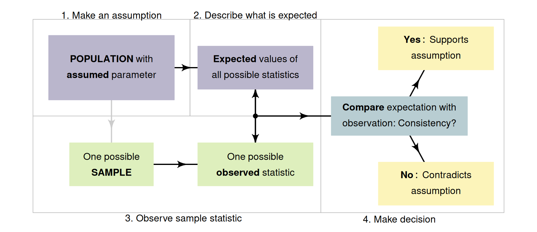
FIGURE 25.1: A way to make decisions.

FIGURE 25.2: A way to make decisions.

This approach is similar to how we unconsciously make decisions every day. For example, suppose I ask my son to brush his teeth (Budgett et al. 2013). Later, I wish to decide if he really did. The decision-making process may proceed as follows.

Assumption: I assume my son brushed his teeth (because I asked him to).
Expectation: based on my assumption, I would expect to find his toothbrush is damp.
Observation: when I check later, I observe a dry toothbrush, which is unexpected.
Decision: the evidence contradicts what I expected to find based on my assumption, so my assumption is probably false: he probably didn't brush his teeth.

I may have made the wrong decision: he may have brushed his teeth, then dried his toothbrush with a hair dryer. However, based on the evidence, he likely has not brushed his teeth.

The situation may have ended differently: when I check later, suppose I observe a damp toothbrush. Then, the evidence seems consistent with what I expected if he brushed his teeth (my assumption), so my assumption is probably true; he probably did brush his teeth. Again, I may be wrong: he may have rinsed his toothbrush under a tap. Nonetheless, I don't have evidence that he didn't brush his teeth.

Similar logic underlies most decision-making in science.⁴

25.4 Making decisions: the steps

Let's think about each step in the decision-making process (Fig. 25.2) individually:

making an assumption about the parameter (Sect. 25.4.1).
describing the expectations of the statistic (Sect. 25.4.2).
taking the sample observations (Sect. 25.4.3).
making a decision (Sect. 25.4.4).

25.4.1 Making an assumption about the parameter

The initial assumption is that sampling variation explains any discrepancy between the values of the parameter and the statistic. This assumption about the value of the parameter is called the null hypothesis, denoted $H_0$.

The null hypothesis is always that sampling variation explains the difference between the observed value of the statistic and the assumed value of the parameter. Depending on the RQ and the context, this may mean:

the parameter value has not changed (e.g., for descriptive or repeated-measures RQs). The value of the statistic might show a change, but only due to sampling variation.
the value of some parameter is the same in all the groups being compared (e.g., for relational RQs). The values of the statistic are not exactly the same due to sampling variation.
there is no relationship between the variables, as measured by some parameter (e.g., for correlational RQs). The value of the statistic is not exactly this value due to sampling variation.

In other words, the null hypothesis is the 'no change, no difference, no relationship' position.

Using this idea, a reasonable assumption can be made about the parameter. For example, when comparing the mean of two groups, we would initially assume no difference between the population means: any difference between the sample means would be attributed to sampling variation.

Example 25.1 (Assumptions about the population) Many dental associations recommend brushing teeth for two minutes. I. D. M. Macgregor and Rugg-Gunn (1979) recorded the toothbrushing time for $85$ uninstructed schoolchildren from England to assess compliance with these guidelines.

We initially assume the population mean toothbrushing time is two minutes ($H_0$: $\mu = 2$). If the sample mean is not two minutes, the null hypothesis explains this discrepancy as sampling variation. A sample can then be obtained to determine if the sample mean is consistent with, or contradicts, this assumption.

25.4.2 Describing the expectations of the statistic

Based on the assumed value for the parameter, we then determine what values to expect from the statistic from all the possible samples we could select (of which we only select one). Since many samples are possible, and every sample is likely to be different (sampling variation), the observed value of the statistic depends on which one of the countless possible samples we obtain. To know what values of the statistic are expected, the sampling distribution needs to be described.

Think about the cards in Sect. 25.1. In a fair pack, half the cards are red in the population (the pack of cards), so the population proportion is assumed to be $p = 0.5$. In a sample of $25$ cards, what values could be reasonably expected for the sample proportion $\hat{p}$ of red cards (the statistic)? If samples of size $n = 25$ were repeatedly taken from a fair pack with $p = 0.5$, the sample proportion of red cards would vary from hand to hand, of course. But how would $\hat{p}$ vary from sample to sample?

Suppose we simulated only ten hands of $n = 25$ cards each, using a computer; the animation below shows the sample proportion of red cards from each repetition. Naturally, the value of $\hat{p}$ varies.

The distribution of the sample statistic is called the sampling distribution (Sect. 19.1). The sampling distribution for $\hat{p}$ is given in Sect. 22.2 when the value of $p$ is known (as assumed here): an approximate normal distribution, with mean $p = 0.5$, and a standard deviation (the standard error) of \[ \text{s.e.}(\hat{p}) = \sqrt{\frac{p\times(1 - p)}{n} } = \sqrt{\frac{0.5\times(1 - 0.5)}{25} } = 0.1. \] A picture of this sampling distribution can be drawn (Fig. 25.3). Values of $\hat{p}$ larger than $0.8$ or smaller than $0.2$ would appear very unlikely.

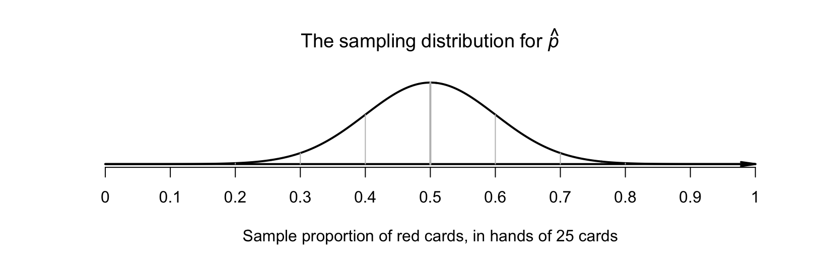
$The sampling distribution for $\hat{p}$, the sample proportion of red cards in $25$ cards.$

FIGURE 25.3: The sampling distribution for $\hat{p}$, the sample proportion of red cards in $25$ cards.

25.4.3 Evaluating the sample observations

While many samples are possible, we only observe one of those countless possible samples. From our sample of $25$ cards, all cards are red (see Sect. 25.1), and so the value of the statistic is $\hat{p} = 25/25 = 1$. Assuming $p = 0.5$, is this value of $\hat{p}$ unusual, or not unusual? From Fig. 25.3, the value $\hat{p} = 1$ is very unusual: it would not be expected in a sample of $25$ cards.

25.4.4 Making a conclusion

Observing $25$ red cards out of $25$ cards from a fair pack is highly unusual, so the chance that our specific, randomly-chosen sample produced $\hat{p} = 1$ is incredibly unlikely. So you could reasonably conclude that finding $\hat{p} = 1$ almost never occurs, if the assumption of a fair pack was true.

But since we did find $\hat{p} = 1$, the assumption of a fair pack is probably wrong. That is, there is persuasive evidence that the assumption is wrong, and that the pack of cards is not fair. The decision-making process is shown in Fig. 25.4.

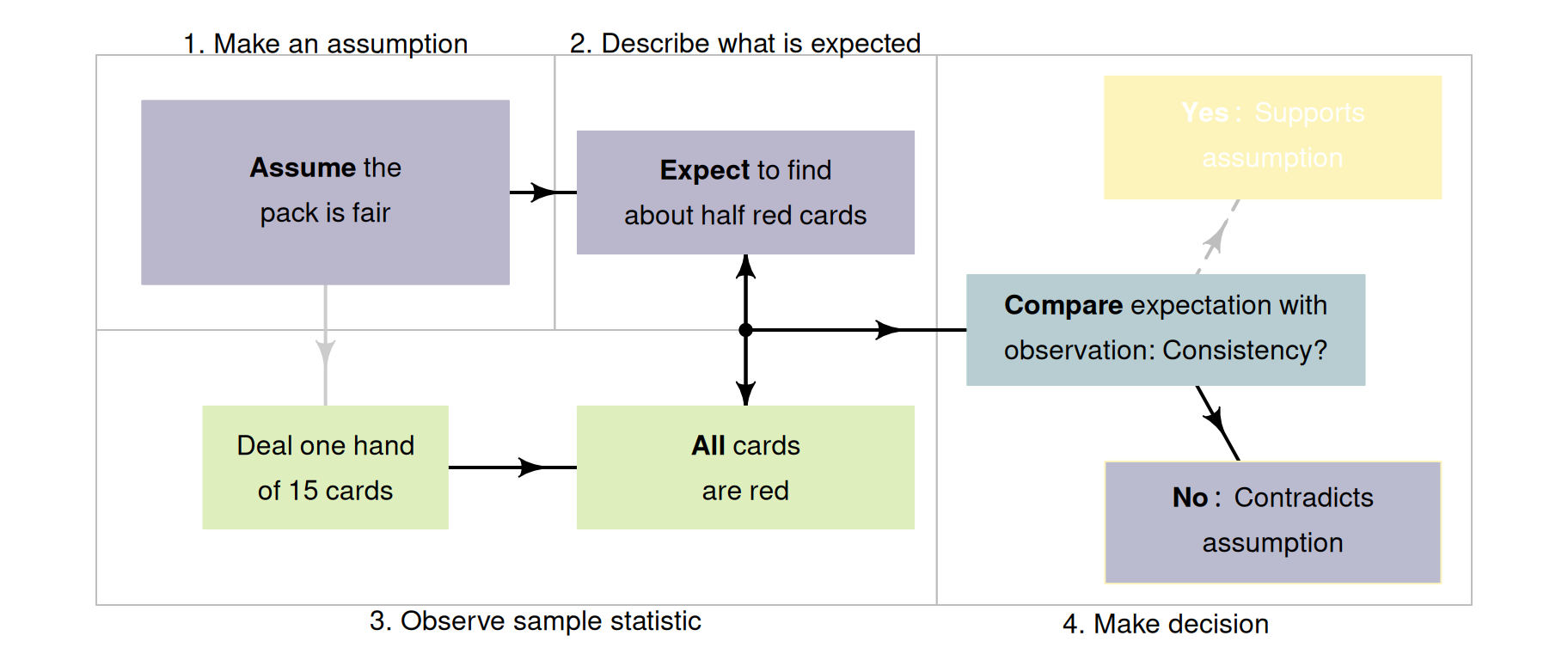
FIGURE 25.4: A way to make decisions for the cards example.

What if we had observed $18$ red cards in a hand of $25$ cards, a sample proportion of $\hat{p} = 18/25 = 0.72$? The conclusion is not quite so obvious then: Fig. 25.3 shows that $\hat{p} = 0.72$ is unlikely, but $\hat{p} = 0.72$ (and even larger values) certainly do occur.

What if $15$ red cards were found in the $25$ (i.e., $\hat{p} = 0.6$)? Figure 25.3 shows that $\hat{p} = 0.6$ could reasonably be observed, since there are many possible samples that lead to $\hat{p} = 0.6$, or even larger values. This would not seem unusual at all, and is certainly not persuasive evidence to change our mind. Many of the possible samples produce values of $\hat{p}$ near $0.6$.

This process of decision-making is similar to the process used in research. This process will be studied in coming chapters.

25.5 Example: brushing teeth

Many dental associations recommend brushing teeth for two minutes (i.e., for $120\,\text{s}$). I. D. M. Macgregor and Rugg-Gunn (1979) recorded the toothbrushing time for $85$ uninstructed schoolchildren from England to assess compliance with these guidelines. Of course, every possible sample of $85$ children in England will include different children, and so produce various sample mean brushing times $\bar{x}$. Even if the population mean toothbrushing time really was $120\,\text{s}$ (i.e., $\mu = 120$), the sample mean probably wouldn't be exactly $120\,\text{s}$, because of this sampling variation.

To begin, assume the population mean toothbrushing time is $\mu = 120$; that is, $H_0$ is $\mu = 120$. If this is true, we then could describe what values of the sample statistic $\bar{x}$ could be expected from all possible samples by describing the sampling distribution of $\bar{x}$: how sample means are likely to vary for samples of size $85$ when $\mu = 120$.

The study found the mean time spent brushing was $60.3\,\text{s}$, with a standard deviation of $23.8\,\text{s}$. Using the ideas in Chap. 23, and in Sect. 23.3 specifically, the sampling distribution of $\bar{x}$ has an approximate normal distribution, with mean $\mu = 120$ (from $H_0$) and a standard deviation of $\text{s.e.}(\bar{x}) = 23.8/\sqrt{85} = 2.58\,\text{s}$ (shown in Fig. 25.5).

A sample mean of $\bar{x} = 60.3$ seems incredibly unlikely if $\mu = 120$. This suggests that the sample evidence contradicts the assumption that $\mu = 120$, and so the mean toothbrushing time in the population is very unlikely to be $120\,\text{s}$.

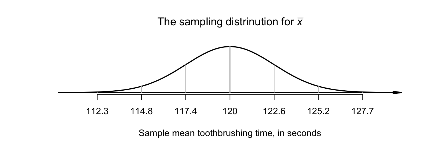
$The sampling distribution for $\bar{x}$, the mean toothbrushing time in schoolchildren from England. A sample mean of $60.3\secs$ seems very unlikely.$

FIGURE 25.5: The sampling distribution for $\bar{x}$, the mean toothbrushing time in schoolchildren from England. A sample mean of $60.3\,\text{s}$ seems very unlikely.

25.6 Chapter summary

Making decisions about parameters based on a statistic is challenging: only one of the many possible samples is observed. Since every sample is likely to be different, different values of the sample statistic are possible. In this chapter, though, a process for making decisions has been studied (Fig. 25.2).

Decisions are often made by making an assumption about the parameter, which leads to an expectation of what values of the statistic are reasonably possible. We can then make observations about our sample, and then make a decision about whether the sample data support or contradict the initial assumption.

25.7 Quick review questions

Are the following statements true or false?

Parameters describe populations.
Both $\bar{x}$ and $\mu$ are statistics.
The value of a statistic is likely to be same in every sample.
Sampling variation describes how the value of a statistic varies from sample to sample.
An initial assumption is made about the sample statistic.
The variation in the value of the statistic from sample to sample is called sampling variation.
If the sample results seem inconsistent with what was expected, then the assumption about the population is probably true.
In the sample, we know exactly what value of $\hat{p}$ to expect.
Hypotheses are made about the population.

25.8 Exercises

Answers to odd-numbered exercises are given at the end of the book.

Exercise 25.1 While playing a die-based game, your opponent rolls a ⚅ ten times in a row.

Do you think there is a problem with the die?
Explain how you came to this decision.

Exercise 25.2 A friend tosses a coin, and obtains H four times in a row.

Do you think there is a problem with the coin?
Explain how you came to this decision.

Exercise 25.3 Since my wife and I have been married, I have been called to jury service four times. The latest notice reads: 'Your name has been selected at random from the electoral roll'.

In the same time, my wife has never been called to jury service. Do you think the selection process really is 'at random'? Explain.

Exercise 25.4 In a 2012 advertisement, an Australian pizza company claimed that their $12$-inch pizzas were 'real $12$-inch pizzas' (P. K. Dunn 2012).

What is a reasonable assumption to make to test this claim?
The claim is supported by a sample of $125$ pizzas, which gave the sample mean pizza diameter as $\bar{x} = 11.48$ inches. What are the two reasons why the sample mean is not exactly $12$-inches?
Does the claim appear to be supported by, or contradicted by, the data? Explain.
Would your conclusion change if the sample mean was $\bar{x} = 11.25$ inches? Explain.
Does your answer depend on the sample size? For example, is observing a sample mean of $11.25$ inches from a sample of size $n = 10$ equivalent to observing a sample mean of $11.25$ inches from a sample of size $n = 125$? Explain.

Exercise 25.5 Suppose that $36$% of all students at a certain large university are aged over $30$. A student takes a sample of $n = 40$ students from the School of Arts to determine if students in that school are somehow different from the general university population in terms of age.

What is the null hypothesis?
If the student researcher finds $13$ students in the sample aged over $30$, does this present persuasive evidence to change your mind? Explain.
If the student researcher finds three students in the sample aged over $30$, does this present persuasive evidence to change your mind? Explain.

24 More details about CIs

26 Hypothesis tests: one proportion