18 Probability

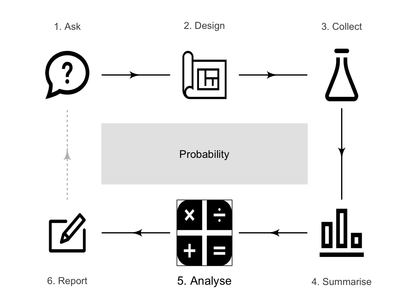
So far, you have learnt to ask a RQ, design a study, and describe and summarise the data. In this chapter, you will learn about probability to describe the random nature of sample statistics. You will learn to:

• explain probability.
• identify and apply various approaches to computing probability.
• determine the probability of events described using and, or and not in simple situations.
• identify events that are independent.
• compute simple conditional probabilities.

18.1 Introduction

This chapter briefly discusses probability. Probability quantifies the chance that a specific, unknown result (an 'event') from some random procedure with an unknown outcome. Before discussing probability, some associated terms needs defining.

18.2 Random procedures, sample spaces and simple events

To talk about probability, a random procedure must be defined first.

Definition 18.1 (Random procedure) A random procedure is a sequence of well-defined steps that (a) can be repeated, in theory, indefinitely under essentially identical conditions; (b) has well-defined results; and (c) has result that are unpredictable for any individual repetition.

Using this definition, the result of rolling a die is a 'random procedure', with possible results ⚀, ⚁, ⚂, ⚃, ⚄ and ⚅.

A list of all distinct possible results from one instance of a random procedure is the sample space. A simple event is any element of the sample space.

Definition 18.2 (Sample space) The sample space is a list of all possible and distinct results after administering a random procedure once.

Definition 18.3 (Simple event) A simple event is a single element of the sample space.

Example 18.1 (Sample spaces) Consider rolling a fair, six-sided die (the random procedure). We do not know what face will be uppermost until we roll the die.

However, the sample space for this procedure can be listed: ⚀, ⚁, ⚂, ⚃, ⚄ and ⚅. These are all mutually exclusive (or distinct) results and cover all possible results (exhaustive), and the sample space is discrete.

The event 'rolling a ⚀' is a simple event.

Combinations of the elements in the sample space are usually of more interest than simple events. These are called compound events.

Definition 18.4 (Compound event) A compound event is any combination of simple events (i.e., of elements in the sample space).

Example 18.2 (Events) Many events can be defined using the sample space in Example 18.1, including:

• Rolling a ⚃: this simple event includes one element of the sample space: ⚃.
• Rolling an odd number: this compound event includes three elements of the sample space: ⚀, ⚂ and ⚄.
• Rolling a number larger than ⚁: this compound event includes four elements of the sample space: ⚂, ⚃, ⚄ and ⚅.

Example 18.3 (Sample spaces and events) Consider the distance you can throw a baseball (the random procedure). We do not know beforehand what distance your next throw will be, but the sample space (the throwing distance) is a number greater than \(0\)(and some of those distances are very unlikely to occur). This sample space is continuous.

Many compound events can be defined using this sample space; for example:

• throwing more than \(50\).
• throwing between \(10\) and \(40\).

Because the sample space is continuous, throwing an exact distance (such as exactly \(10\)) is technically not possible.

Events of interest are often related to other events, using and, or, not. Consider two events called \(A\) and \(B\). Then, '\(A\) and \(B\)' is the event comprising events in \(A\) and also in \(B\). (In other words, events in both \(A\) and \(B\).) '\(A\) or \(B\)' is the event comprising events in \(A\), events in \(B\), and events in both. The event 'not \(A\)' comprises all the events in the sample space that are not in Event \(A\).

Example 18.4 (Complicated events) Consider rolling a fair, six-sided die again (Example 18.1). Suppose these two (compound) events are defined:

• Event \(A\): Roll a number divisible by \(2\).
• Event \(B\): Roll a number divisible by \(3\).

Event \(A\) comprises the simple events roll a ⚁, roll a ⚃ and roll a ⚅, and event \(B\) comprises the simple events roll a ⚂ and roll a ⚅.

Then, the event '\(A\) and \(B\)' includes all events in \(A\) and also in \(B\); that is, '\(A\) and \(B\)' comprises the single simple event roll a ⚅.

Event '\(A\) or \(B\)' include the events in \(A\), the events in \(B\), and those in both; that is, '\(A\) or \(B\)' comprises the four simple events roll a ⚁, roll a ⚂, roll a ⚃ and roll a ⚅.

The event 'not \(A\)' comprises the three simple events roll a ⚀, roll a ⚂ and roll a ⚄.

18.3 Probability

Using these definitions, a probability can be defined.

Definition 18.5 (Probability) A probability is a number between \(0\) and \(1\) inclusive (or between \(0\)% and \(100\)% inclusive) that quantifies the likelihood of a certain event occurring.

A probability of \(0\) (or \(0\)%) means the event is 'impossible' (will never occur), and a probability of \(1\) (or \(100\)%) means that the event is certain to happen (will always occur). Most events have a probability between the extremes of \(0\)% and \(100\)%.

Example 18.5 (Probabilities) Consider these cases:

• The probability of receiving negative rainfall is \(0\); it is impossible.
• The probability of receiving some rain in London next year is \(1\); it is certain.
• The probability of receiving rain on a specific day in London next year is between \(0\) and \(1\) inclusive.

18.4 Determining probabilities

The probability of an event occurring can be determined in different ways, including:

• the classical approach (Sect. 18.4.1);
• the relative frequency approach (Sect. 18.4.2); and
• the subjective approach (Sect. 18.4.3).

18.4.1 Classical approach

What is the probability of rolling a ⚃ on a die? The sample space has six possible outcomes (see Example 18.1) that are equally likely to occur, and the event 'rolling a ⚃' comprises just one of those events. Thus,

\[ \text{Probability of rolling a 4} = \frac{\text{The number of results that are a 4}}{\text{The number of possible results}} = \frac{1}{6}. \]

This approach to computing probabilities is called the classical approach to probability, and is only appropriate when all events in the sample space are equally likely.

Definition 18.6 (Classical approach to probability) In the classical approach to probability, the probability of an event occurring is the number of elements of the sample space included in the event, divided by the total number of elements in the sample space, when all outcomes are equally likely.

By this definition: \[ \text{Prob. of an event} = \frac{\text{Number of results in the event of interest}}{\text{Total number of equally-likely results}}. \]

We can say that 'the probability of rolling a ⚃ is \(1/6\)', or 'the probability of rolling a ⚃ is (approximately) \(0.1667\)'. The answer can also be expressed as a percentage: 'the probability of rolling a ⚃ is (approximately) \(16.67\)%'. The answer could also be interpreted as 'the expected proportion of rolls that are a ⚃ is (approximately) \(0.1667\)'. That is, about \(16.67\)% of a very large number of future rolls are likely to be a ⚃.

The chance of rolling a ⚃ is \(0.1667\), but any single roll of the die either will or will not produce a ⚃, and we don't know which will occur.

Example 18.6 (Complicated probabilities) Consider rolling a standard six-sided die. With six equally-likely results (Example 18.1), each with probability \(1/6\) (or, approximately, \(16.67\)%) of occurring, the probability of rolling an even number is \(3/6\), since there are three even numbers in the sample space.

Example 18.7 (Describing probability) Consider rolling a standard six-sided die.

• The probability of rolling an even number is \(3 \div 6 = 0.5\).
• The percentage of rolls expected to be even is \(3 \div 6 \times 100 = 50\)%.
• The odds of rolling an even number is \(3\div 3 = 1\).

Example 18.8 (Events) The probability of the events listed in Example 18.2 are:

• The probability of rolling a ⚃ is \(1/6\) (or about \(0.1667\)).
• The probability of rolling an odd number is \(3/6\), or \(1/2\) (or \(0.5\)).
• The probability of rolling a number larger than ⚁ is \(4/6\), or \(2/3\) (or about \(0.6667\)).

Probabilities describe the likelihood that an event will occur before the result is known. Odds and proportions can be used either before or after the result is known, provided the wording is correct.

For example, proportions describe how often an event has occurred after the result is known, and expected proportions describe the likelihood that an event will occur in a large number of repetitions before the result is known.

The following example may help explain.

Example 18.9 (Probabilities, proportions and odds) Before a fair coin is tossed:

• The probability of throwing a head is \(1/2 = 0.5\) (or \(50\)%).
• The expected proportion of heads for many coin tosses is \(0.5\).
• The odds of throwing a head is \(1/1 = 1\).

If we have already tossed a coin \(100\) times and found \(47\) heads:

• The proportion of heads in the sample is \(47/100 = 0.47\) (or \(47\)%).
• The odds that we threw a head in the sample is \(47/53 = 0.887\).

The 'probability that we just threw a head' makes no sense, because the result is known.

18.4.2 Relative frequency approach

What is the probability that a new-born baby will be a boy? The sample space could be listed as: boy and non-boy. Since the sample space has two elements, the classical approach suggests the probability is \(1\div2 = 0.5\). However, this approach is appropriate only if boys and non-boys are equally likely to be born. But are they?

In Australia in 2021, \(289\ 603\) live births occurred, with \(148\ 636\) male births, \(140\ 944\) female births, and \(23\) others (or 'not stated'). The proportion of boys born in 2021 is \(148\ 636\div 289\ 603 = 0.513\), or about \(51.3\)%. An estimate of the probability that the next birth will be a boy is about \(0.513\) (or \(51.3\)%), based on past data. This is the relative frequency approach to calculating probabilities: using past data.

Using the relative frequency method can only ever produce an approximate probability, as it is based on a limited number of past observations. An actual probability would require an infinite number of observations.

Definition 18.7 (Relative frequency approach to probability) In the relative frequency approach to probability, the probability of an event is approximately the number of times the outcomes of interest has appeared in the past, divided by the number of 'attempts' in the past. This produces an approximate probability.

Example 18.10 (Relative frequency probability) Based on the earlier information, the odds that a new baby will be a boy is approximately \(0.513\div (1 - 0.513) = 1.053\). According to the Australian Bureau of Statistics (ABS):

The sex ratio for all births registered in Australia generally fluctuates around \(105.5\) male births per \(100\) female births.

This is close to the odds of \(1.053\) found above.

18.4.3 Subjective approach

Many probabilities cannot be computed using the classical or relative frequency approach; for example, what is the probability that your sporting team wins their next game? In this case, only a subjective probability can be given.

'Subjective' probabilities may be based on personal judgement or experience. They can also be given by considering all the relevant issues that may impact the probability (and may, for example, be based on mathematical models that incorporate information from numerous inputs). Depending on how these other issues are considered and combined, different subjective probabilities may be given.

Weather forecasts are one example: they incorporate data from sea surface temperatures, local topography, air pressures, air temperatures and so on. Different models use different inputs, and may combine these inputs differently to produce different (subjective) forecast probabilities.

Definition 18.8 (Subjective approach to probability) In the subjective approach to probability, various factors are incorporated, perhaps subjectively, to determine the probability of an event occurring.

Example 18.11 (Subjective probability) During El Niño events, eastern Australia typically experiences drier-than-average winters and springs. The Australian Broadcasting Corporation's news website reported (on 23 May, 2023) that the Australian Bureau of Meteorology predicted a \(50\)% probability of an El Niño event in 2023, while the American National Oceanic and Atmospheric Administration predicted a \(90\)% chance of an El Niño event in 2023.

Despite this, '[both] agencies are looking at the same part of the Pacific Ocean' to make their predictions. However, 'the US and Australia base their probability on different criteria'. The probabilities are subjective probabilities, based on complex mathematical models.

18.5 Independence

One important concept in probability is independence. Two events are independent if the probability of one event happening is the same, whether or not the other event has happened. For example, if you toss a coin, the probability of getting a head is the same whether you are sitting or standing. That is, the result of a coin toss is independent of your position.

Definition 18.9 (Independence) Two events are independent if the probability of one event is the same, whether or not the other event has happened.

Example 18.12 (Independence) Consider drawing two cards from a fair pack (of \(52\) cards), without returning the first card. For the first card, the sample space contains every card in the pack, and drawing any one card is as equally likely as drawing any other. Since four cards are Aces, the probability of drawing an Ace on the first draw is \(4/52\) (using the classical approach).

If we drew an Ace for the first card, the probability of drawing an Ace for the second card is \(3/51\) (three Aces remain among the \(51\) remaining cards). Alternatively, if we don't draw an Ace for the first card, the probability of drawing an Ace second time is \(4/51\) (four Aces remain among the \(51\) remaining cards).

That is, the probability of drawing an Ace for the second card depends on whether or not an Ace was drawn for the first card. The two events 'Drawing an Ace for the first card' and 'Drawing an Ace for the second card' are not independent events.

A 'standard' pack of cards has \(52\) cards, organised into four suits: spades \(\spadesuit\), clubs \(\clubsuit\) (both black), hearts \(\heartsuit\) and diamonds \(\diamondsuit\) (both red). Each suit has \(13\) denominations: \(2\), \(3\), \(4\), \(5\), \(6\), \(7\), \(8\), \(9\), \(10\), Jack (J), Queen (Q), King (K), Ace (A). The Ace, King, Queen and Jack cards are called picture cards. (Most packs also contain two jokers, which are not considered part of a standard pack.)

Random samples produce independent units of analysis.

18.6 Conditional probability

Conditional probability refers to adjusting probabilities when extra information is known. For example, the probability of rolling a ⚀ is \(1/6\) using the classical approach, as the sample space has six elements. However, if we are told that the number rolled is a odd number, only three elements in the sample space need now be considered, rather than six: ⚀, ⚂, ⚄. No other outcomes are possible, and so the probability or rolling a ⚀ is \(1/3\). We say 'the probability of rolling a ⚀, given that the roll is an odd number, is \(1/3\)'.

Example 18.13 (Conditional probability) Suppose someone draws a card from a pack of cards. The probability that the card is a \(\clubsuit\) is \(13/52 = 1/4\), or \(25\)%.

However, if that person tells you that the card is a black card, then the card must be either a \(\clubsuit\) or \(\spadesuit\). Hence, the probability that the card is a \(\clubsuit\), given that the card is black, is \(13/26 = 1/2\), or \(50\)%.

Example 18.14 (Wearing sunglasses) B. Dexter et al. (2019) recorded the number of people at the foot of the Goodwill Bridge, Brisbane, who wore sunglasses between \(11\):\(30\)am to \(12\):\(30\)pm (Table 18.1). The probability of an observed person wearing sunglasses is \[ \frac{126 + 123}{126 + 123 + 240 + 263} = 0.3311, \] or about \(33.1\)%.

We can also compute conditional probabilities:

• If the observed person is female, the probability that she is wearing sunglasses is \(126\div (240 + 126) = 0.3443\), or about \(34.4\)%.
• If the observed person is male, the probability that he is wearing sunglasses is \(123\div (263 + 123) = 0.3187\), or about \(31.9\)%.

These probabilities are close, but not exactly equal.

If the two events were independent, then these two conditional probabilities would be the same: the probability of wearing sunglasses would be the same for females and males. In other words, the probability of wearing sunglasses did not depend on whether we were observing a female or a male. We might say that wearing sunglasses is close to, but not exactly, independent of the sex of the person, in the sample. We cannot be sure if wearing sunglasses in independent of the sex of the person in the population.

TABLE 18.1: Females and males wearing sunglasses on the Goodwill Bridge, Brisbane.

	Female	Male
Not wearing sunglasses	\(240\)	\(263\)
Wearing sunglasses	\(126\)	\(123\)

18.7 Chapter summary

Three ways to compute probabilities are:

• the classical approach, which requires all outcomes to be equally likely;
• the relative frequency approach (giving approximate probabilities); and
• the subjective approach.

Two events are independent if the probability of one event is the same, whether or not other event has happened. Conditional probability incorporate extra information when the probability is computed.

18.8 Quick review questions

Suppose Event \(A\) is defined as 'Rolling a ⚀ or a ⚁ on a fair die'. Also, suppose Event \(B\) is defined as 'Rolling an even number on a die'.

1. What is the best approach to computing the probability of Event \(A\) occurring?
   The classical approachThe relative frequency approachThe subjective approach
2. What is the probability of Event \(A\) occurring?
   1/6 2/6 1/5 2/5 5/2 5/1
3. True or false: Events \(A\) and \(B\) are independent.
   TRUE FALSE
4. What is the probability of '\(A\) and \(B\)' occurring?
   0 1/6 2/6 3/6 4/6 5/6 1
5. What is the probability of '\(A\) or \(B\)' occurring?
   0 1/6 2/6 3/6 4/6 5/6 1
6. What is the probability of 'not \(B\)' occurring?
   0 1/6 2/6 3/6 4/6 5/6 1
7. What are the odds of 'not \(B\)' occurring?
   0 1/6 2/6 3/6 4/6 5/6 1

18.9 Exercises

Answers to odd-numbered exercises are available in App. E.

Exercise 18.1 Which approach is best used to estimate a probability in these situations?

1. The probability that the stock market will rise next month.
2. The probability that a randomly-chosen person writes left-handed.

Exercise 18.2 Which approach is best used to estimate a probability in these situations?

1. The probability that a King will be chosen from a pack of cards.
2. The probability that Paris receives more than \(50\)of rain next May.

Exercise 18.3 Consider drawing cards from a fair pack. Event A is 'drawing a picture card', Event B is 'drawing a King or Ace' and Event C is 'drawing a \(\spadesuit\).

1. What events are in '\(A\) and \(B\)'?
2. Compute the probability of '\(A\) and \(B\)'.
3. What events are in '\(A\) or \(B\)'?
4. Compute the probability of '\(A\) or \(B\)'.
5. What events are in '\(A\) and \(C\)'?
6. Compute the probability of '\(A\) and \(C\)'.
7. What events are in 'not \(C\)'?
8. Compute the probability of 'not \(C\)'.
9. Compute the probability of \(C\), if \(A\) has already occurred.
10. Compute the probability of \(A\), if \(C\) has already occurred.

Exercise 18.4 Consider rolling a fair die. Event A is 'rolling a an even number', Event B is 'rolling an odd number' and Event C is 'rolling a ⚁'.

1. What events are in '\(A\) and \(B\)'?
2. Compute the probability of '\(A\) and \(B\)'.
3. What events are in '\(A\) or \(B\)'?
4. Compute the probability of '\(A\) or \(B\)'.
5. What events are in '\(A\) and \(C\)'?
6. Compute the probability of '\(A\) and \(C\)'.
7. What events are in 'not \(C\)'?
8. Compute the probability of 'not \(C\)'.
9. Compute the probability of \(C\), if \(A\) has already occurred.
10. Compute the probability of \(C\), if \(B\) has already occurred.

Exercise 18.5 Consider these three events about tossing two fair coins, say Coin A and Coin B: Event 1 is 'toss a Head on Coin A'; Event 2 is 'toss a Tail on Coin A'; and Event 3 is 'toss a Head on Coin B'.

1. Are Event 1 and Event 2 independent events?
2. Are Event 1 and Event 3 independent events?
3. Compute the probability of Event 3.
4. What is the probability of Event 3 occurring, if Event 1 has already occurred?
5. List the sample space for the random procedure.

Exercise 18.6 Consider these three events about drawing one card from a fair pack: Event 1 is 'draw a Jack'; Event 2 is 'draw a \(\heartsuit\)'; and Event 3 is 'draw a \(\clubsuit\)'.

1. Compute the probability of Event 1.
2. Compute the probability of Event 1, if Event 2 has occurred.
3. Compute the probability of Event 1, if Event 2 has not occurred.
4. Are Event 1 and Event 2 independent? Explain.
5. Compute the probability of Event 3.
6. Compute the probability of Event 3, if Event 2 has occurred.
7. Compute the probability of Event 3, if Event 2 has not occurred.
8. Are Event 2 and Event 2 independent? Explain.

Exercise 18.7 Suppose I roll a standard six-sided die.

1. What is the probability that I will roll a number larger than ⚁? 0 1/6 2/6 3/6 4/6 5/6 1

2. What are the odds of rolling a number smaller than ⚅? 0 1/6 1/5 5/6 6/5 5 5/6 1

3. Suppose I toss a coin after rolling the die. Is the result from the coin toss independent of what I rolled on the die?

   No: because there are six possible outcomes from rolling a die, but only two from tossing a coinYes: because die was not rolled at the same time as the coin was tossedYes: what happens on the die won't change what happens on the coinNo: because the die was not rolled at the same time as the coin was tossed

4. What is the probability that I roll a number divisible by \(2\) on the die? 0 1/6 2/6 3/6 4/6 5/6 1

5. What is the probability that I roll a number divisible by \(2\) and divisible by \(3\) on the die? 0 1/6 2/6 3/6 4/6 5/6 1

6. What is the probability of rolling a ⚁, given that the number is smaller than ⚃?

Exercise 18.8 Suppose you have a well-shuffled, standard pack of \(52\) cards.

1. What is the probability that you will draw a King?
2. What are the odds that you will draw a King?
3. What is the probability that you will draw a picture card (Ace, King, Queen or Jack)?
4. What are the odds that you will draw a picture card (Ace, King, Queen or Jack)?
5. Suppose I draw two cards from the pack. Are the events 'Draw a King first' and 'Draw a Queen second' independent events?
6. Suppose I draw one card from the pack, then roll a six-sided die. Are the events 'Draw a Jack from the pack of cards' and 'Roll a ⚄ on the die' independent events?
7. If I draw a picture card, what is the probability the card is a King?

Exercise 18.9 Consider drawing a card from a standard, well-shuffled pack of cards. The first card is replaced, the pack reshuffled, and then a second card is drawn from the pack. The colour of the two cards is recorded (B: Black; R: Red), and we are interested in Event \(D\): 'the total number of black cards drawn, minus the total number of red cards drawn'.

1. Write down the sample space.
2. Find the probability that \(D\) is zero.
3. Find the probability that \(D\) is zero or one.
4. Is the colour of the card drawn first independent of the colour of the card drawn second? Explain.

Exercise 18.10 Consider the random process ‘tossing a coin until a Head is observed’. Event \(H\) is of interest: 'the number of tosses until the first head is thrown’.

1. What is the sample space?
2. Find the probability that \(H\) is one.
3. Find the probability that \(H\) is two.
4. Find the probability that \(H\) is one or two.

Exercise 18.11 P. K. Dunn (2023) tabulated information about school children in Queensland in 2019 (Table 18.2).

1. What is the probability that a randomly chosen student is a first-nations student?
2. What is the probability that a randomly chosen student is in a government school?
3. Is the sex of the student approximately independent of whether the student is a first nations student, for students in government schools?
4. Is the sex of the student approximately independent of whether the student is a first nations student, for students in non-government schools?
5. Is the sex of the student approximately independent of the type of school, for female students?
6. Is the sex of the student approximately independent of the type of school, for male students?
7. Based on the above, what can you conclude from the data?

TABLE 18.2: The number of first nation and non-first nation students in Queensland schools in 2019.

	Number of first nations students	Number of non-first nations students
Government schools
Females	\(2\,540\)	\(21\,219\)
Males	\(2\,734\)	\(22\,574\)
Non-government schools
Females	\(\phantom{0}391\)	\(\phantom{0}9\,496\)
Males	\(\phantom{0}362\)	\(\phantom{0}9\,963\)

Exercise 18.12 Kelishadi et al. (2017) recorded whether Iranian children aged \(6\)--\(18\) years ate breakfast (Table 18.3) Find the probability that a randomly chosen student is:

1. A female student.
2. A female student who skipped breakfast.
3. A female student, if we already know the child skipped breakfast.

TABLE 18.3: The number of Iranian children aged \(6\) to \(18\) who skip and do not skip breakfast.

	Skips breakfast	Doesn't skip breakfast	Total
Females	\(2\,383\)	\(4\,257\)	\(\phantom{0}6\,640\)
Males	\(1\,944\)	\(4\,902\)	\(\phantom{0}6\,846\)
Total	\(4\,327\)	\(9\,159\)	\(13\,486\)

Exercise 18.13 Are these pairs of events likely to be independent or not independent? Explain.

1. 'I walk to work tomorrow morning', and 'Rain is expected tomorrow morning'.
2. 'A person smokes more than \(10\) cigarettes per week' and 'A person gets lung cancer'.
3. 'It rains today' and 'I hose my garden today'.

Exercise 18.14 In disease testing, two keys aspects of the test are:

• Sensitivity: the probability of a positive test result among those with the disease; and
• Specificity: the probability of a negative test result among those without the disease.

Both are important for understanding how well a test works in practice. Ideally, a test would have high sensitivity and high specificity.

A certain test has a sensitivity of \(0.99\) and a specificity of \(0.98\). Consider a group of \(1\,000\) people, \(100\) of whom (unknowingly) have the disease and \(900\) who (unknowingly) do not have the disease. All the people are given the test.

1. Suppose the \(100\) people who do have a disease are tested. How many would be expected to return a positive test result?
2. Suppose the \(900\) people who do not have a disease are tested. How many would be expected to return a positive test result?
3. In total, how many positive tests would be expected from the \(1000\) people?
4. Consider those people who return a positive test result. What is the probability that one of these people actually has the disease?

Exercise 18.15 Explain why the following argument is incorrect:

When I toss two coins, there are only three outcomes: a Head and a Head, a Tail and a Tail, or one of each. So the probability of obtaining two Tails must be one-third.

Exercise 18.16 On October 13, the American television programme Nightline interviewed Dr Richard Andrews, director of the California Office of Emergency Services, to discussed various natural disasters that were being predicted. In the interview, Dr Andrews said:

I listen to earth scientists talk about earthquake probabilities a lot and in my mind every probability is \(50\)--\(50\), either it will happen or it won't happen.

Explain why Dr Andrews is incorrect when he says that 'every probability is \(50\)--\(50\)'. Give an example to show why he must be incorrect. (Based on a report in Chance News 6.12.)

---

Peter K. Dunn, 2024: CC BY-NC-SA 4.0