22 Confidence intervals: one proportion
So far, you have learnt to ask an RQ, design a study, describe and summarise the data, and model sampling variation. In this chapter, you will learn to construct confidence intervals for one proportion. You will learn to:
- identify situations where estimating a proportion is appropriate.
- form confidence intervals for one proportion.
- determine whether the conditions for using the confidence intervals apply in a given situation.
22.1 Introduction
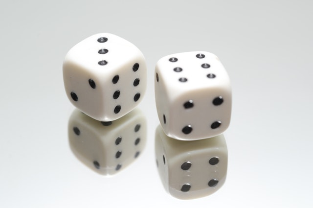
Suppose a fair, six-sided die is rolled \(25\) times. What proportion of the rolls will produce an even number? That is, what will be the value of the sample proportion of numbers that are even? Of course, no-one knows, because the proportion of rolls that will be even will not be the same for every sample of \(25\) rolls. The value of the sample proportion (the statistic) varies from sample to sample: sampling variation exists.
22.2 Sampling distribution for \(\hat{p}\): for \(p\) known
As seen in Chap. 19, sample statistics often vary with a normal distribution (whose standard deviation is called the standard error). However, being more specific about the details of the normal distribution (such as the values of its mean and standard deviation) is useful.
Remember: studying a sample leads to the following observations:
- every sample is likely to be different.
- we observe just one of the many possible samples.
- every sample is likely to yield a different value for the statistic.
- we observe just one of the many possible values for the statistic.
Since many values for the sample proportion are possible, the values of the sample proportion vary (called sampling variation) and have a distribution (called a sampling distribution).
To better understand the sampling distribution for the proportion of even numbers in \(25\) rolls of a die, statistical theory could be used, or thousands of repetitions of a sample of \(25\) rolls could be performed, or a computer could simulate many samples of \(25\) rolls (like we did for a roulette wheel in Sect. 19.2).
Here, the population proportion of even rolls is \(p = 0.5\) (using the classical approach to probability: three of the six faces of the die are even). Each sample of \(n = 25\) rolls produces a sample proportion, denoted by \(\hat{p}\), which varies from sample to sample.
\(p\) refers to the population proportion, and \(\hat{p}\) refers to a sample proportion.
The sample proportions would be expected to vary around \(p = 0.5\) (the population proportion): some values of \(\hat{p}\) larger than \(p\), and some smaller than \(p\). The value of the sample proportion in \(25\) rolls could be very small or very high by chance, but we wouldn't expect to see that very often. The sample proportions exhibit sampling variation, and the amount of sampling variation is quantified using a standard error.
Suppose a fair die was rolled \(25\) times, and this random procedure was repeated thousands of times, and the proportion of even rolls was recorded for every one of those thousands of sets of \(25\) rolls. These thousands of sample proportions \(\hat{p}\) (one from every sample of \(n = 25\) rolls) could be shown using a histogram; see the animation below.
The shape of the histogram is roughly a normal distribution. The sampling distribution for \(\hat{p}\) will always have an approximately normal distribution when certain conditions are met: see Sect. 22.7. The mean of this distribution is called the sampling mean, and the standard deviation for this sampling distribution is called the standard error, denoted \(\text{s.e.}(\hat{p})\) (see Fig. 22.1).
More specifically, the values of the mean and standard deviation of the normal distribution the animation above can be determined:
- the sampling mean has the value of \(p = 0.5\) (i.e., the average value of \(\hat{p}\) is \(0.5\)).
- the standard deviation, called the standard error \(\text{s.e.}(\hat{p})\), has the value \(0.1\). (The source of this number will be revealed soon, in Equation (22.2).)
This distribution is the sampling distribution, whose standard deviation is called a standard error. A picture of this normal distribution can be drawn (Fig. 22.1). While we still don't know exactly what the next roll will produce, we have some idea of how the sample proportion varies in samples of \(25\) rolls. For instance, values of \(\hat{p}\) less than \(0.2\), or greater than \(0.8\) are unlikely to be observed from a fair die (with \(p = 0.5\)) in \(25\) rolls.
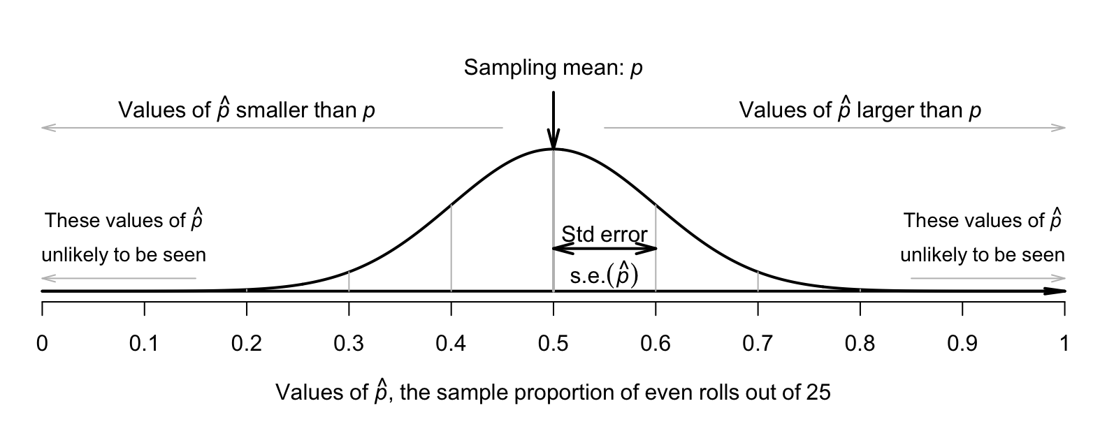
FIGURE 22.1: The sampling distribution is an approximate normal distribution with mean \(0.5\) and standard error \(0.1\); it is a model for how the proportion of even rolls varies when a die is rolled \(25\) times.
More generally, the sampling distribution of \(\hat{p}\) is described as follows.
Definition 22.1 (Sampling distribution of a sample proportion with population proportion known) When the value of \(p\) is known, the sampling distribution of the sample proportion is (when certain conditions are met; Sect. 22.7) described by
- an approximate normal distribution,
- centred around the sampling mean whose value is \(p\),
- with a standard deviation (called the standard error of \(\hat{p}\)), whose value is \[\begin{equation} \text{s.e.}(\hat{p}) = \sqrt{\frac{ p \times (1 - p)}{n}}, \tag{22.1} \end{equation}\] where \(n\) is the size of the sample used to compute \(\hat{p}\), and \(p\) is the population proportion.
The parameter \(p\) and the statistic \(\hat{p}\) are both proportions. However, the average value of the sample proportions from all possible samples can be described by a sampling mean, whose value is \(p\). The sampling mean of the sampling distribution is the 'average' value of all possible sample proportions, \(\hat{p}\).
For the die example, where \(n = 25\) rolls and \(p = 0.5\), using Equation (22.1) gives: \[\begin{equation} \text{s.e.} (\hat{p}) = \sqrt{\frac{0.5 \times (1 - 0.5)}{25}} = 0.1. \tag{22.2} \end{equation}\] This standard error is the standard deviation of the normal distribution in the animation in Sect. 22.2.
In practice the value of \(p\) is almost always unknown. This situation is studied from Sect. 22.4 onwards.
22.3 Sampling intervals for \(\hat{p}\)
Since the possible values of the sample proportions \(\hat{p}\) can be described by an approximate normal distribution, the \(68\)--\(95\)--\(99.7\) rule (Def. 20.1) applies.
For example, in Fig. 22.1 (where the sampling mean is \(0.5\) and the standard error is \(0.1\)), about \(68\)% of the time a sample of \(25\) rolls will have a value of \(\hat{p}\) between \(0.5\) give-or-take one standard deviation (that is, give-or-take \(0.1\)).
So, about \(68\)% of the time, the proportion of even rolls in a sample of \(25\) rolls will lie between \(0.5 - 0.1 = 0.4\) and \(0.5 + 0.1 = 0.6\). Similarly, about \(95\)% of the time, the proportion of even rolls will be between \(0.5\) give-or-take \((2\times0.1\)), or between \(0.3\) and \(0.7\).
These intervals tell us what values of \(\hat{p}\) are likely to be observed in samples of size \(25\). Most of the time (i.e., approximately \(95\)% of the time), the value of \(\hat{p}\) is expected to be between \(0.30\) and \(0.70\) (Fig. 22.2).
Formally, the sample proportion \(\hat{p}\) is likely to lie within the interval \[ p \pm \big(\text{multiplier} \times \text{s.e.}(\hat{p})\big), \] where \(\text{s.e.}(\hat{p})\) is the standard error of the sample proportion (calculated using Equation (22.1)). The multiplier is a \(z\)-score, whose value depends on how confident we wish to be that the interval contains the value of \(\hat{p}\). For a \(95\)% interval, the multiplier is approximately \(2\), based on the \(68\)--\(95\)--\(99.7\) rule: approximately \(95\)% of observations are within two standard deviations of the value of \(p\) (the mean of the normal distribution in Fig. 22.1). That is, the approximate \(95\)% sampling interval is: \[ p \pm (2 \times \text{s.e.}(\hat{p}) ). \] An exact value for the multiplier (i.e., a \(z\)-score) can be found using Appendix B.1. Any level of confidence can be used (but different multipliers are then needed). This interval is called a sampling interval.
The symbol '\(\pm\)' means 'plus or minus', or (colloquially) 'give-or-take'.
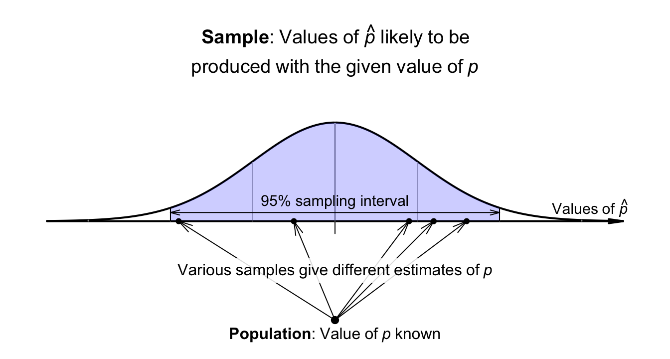
FIGURE 22.2: A known value of \(p\) produces a range of \(\hat{p}\) values.
22.4 Sampling distribution for \(\hat{p}\): for \(p\) unknown
In the die example (Sects. 22.2 and 22.3), the value of \(p\) was known. However, usually the value of \(p\) (the parameter) is unknown; after all, the reason for taking a sample is to estimate the unknown value of \(p\). When the value of \(p\) is unknown, the standard error is computed using the best available estimate of \(p\), which is \(\hat{p}\).
Definition 22.2 (Sampling distribution of a sample proportion with population proportion unknown) When the value of \(p\) is unknown, the sampling distribution of the sample proportion is (when certain conditions are met; Sect. 22.7) described by
- an approximate normal distribution,
- centred around the sampling mean, whose value is \(p\),
- with a standard deviation (called the standard error of \(\hat{p}\)) whose value is \[\begin{equation} \text{s.e.}(\hat{p}) = \sqrt{\frac{ \hat{p} \times (1 - \hat{p})}{n}}, \tag{22.3} \end{equation}\] where \(n\) is the size of the sample used to compute \(\hat{p}\), and \(\hat{p}\) is the sample proportion. In general, the approximation gets better as the sample size gets larger.
When computing the standard error for a proportion, take care! Make sure you use a proportion in the formula, not a percentage (i.e., \(0.5\) rather than \(50\)%). Also: don't forget to take the square root.
22.5 Confidence intervals for \(p\)
Let's pretend for the moment that the population proportion of even rolls on a die is unknown (simply to demonstrate ideas). An estimate of the population proportion of even rolls could be found by rolling a die \(n = 25\) times, and computing \(\hat{p}\) (an estimate of \(p\)). Suppose \(11\) of the \(n = 25\) rolls produce an even number, so \(\hat{p} = 11/25 = 0.44\). The best estimate of \(p\) is therefore \(\hat{p} = 0.44\). We might expect the (unknown) value of \(p\) to be a little smaller than this estimate \(\hat{p}\), or a little larger.
Using Def. 22.2, the sample proportions vary with an approximate normal distribution around \(p\) (whose value is unknown), with a standard deviation (the standard error) of \[ \text{s.e.}(\hat{p}) = \sqrt{\frac{ 0.44 \times (1 - 0.44)}{25}} = 0.09927739. \] Previously, the sampling distribution was used to construct a sampling interval that was likely to contain the unknown value of \(\hat{p}\). However, here the value of \(\hat{p}\) is known, so an interval is created that is likely to contain the unknown value of \(p\) that produced the observed value of \(\hat{p}\) (Fig. 22.3).
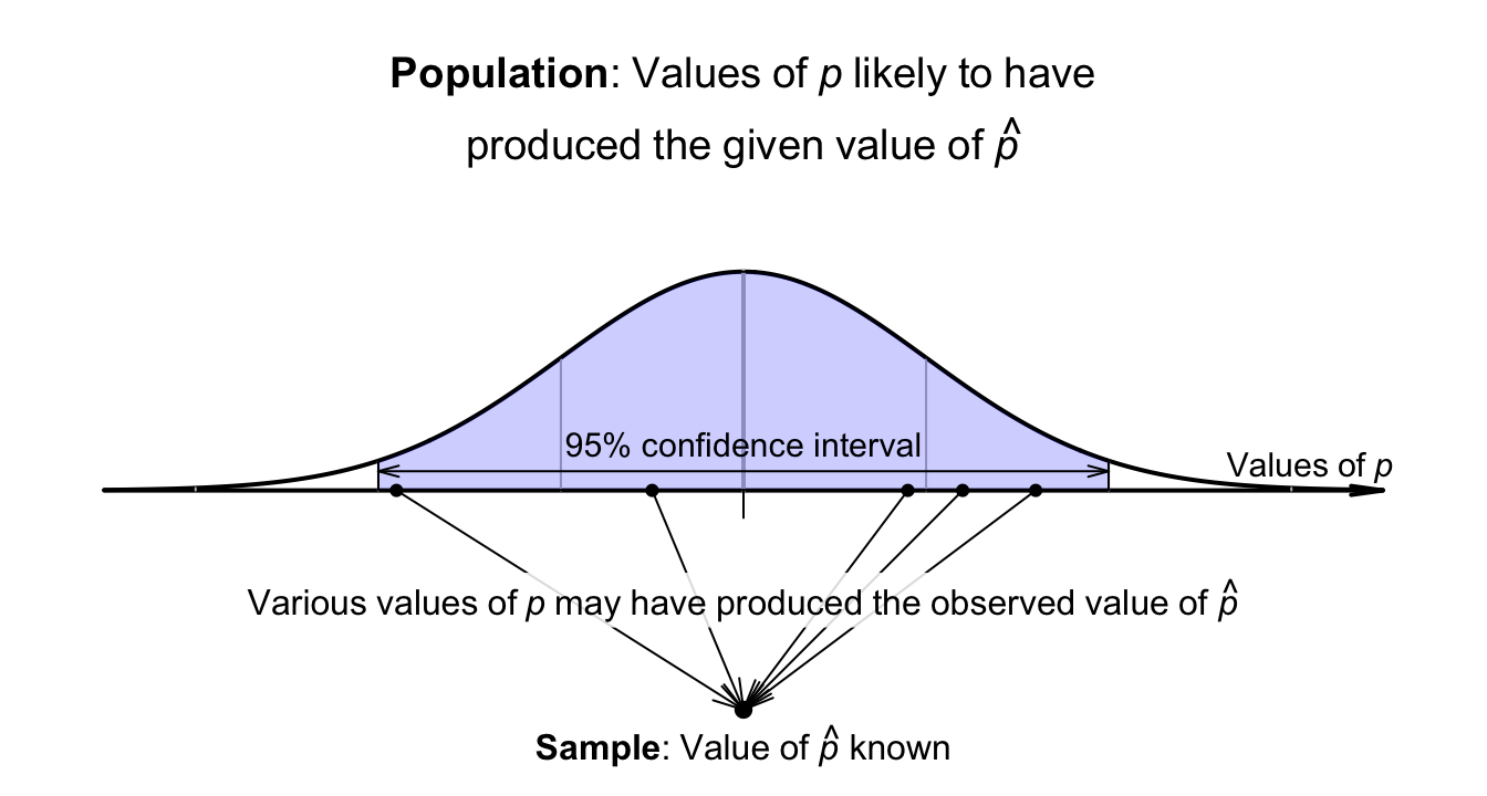
FIGURE 22.3: The sampling distribution for \(\hat{p}\): many values of \(p\) may have produced the observed value of \(\hat{p}\).
The unknown value of \(p\) could be a little smaller or a little larger than the value of \(\hat{p}\); the interval is the value of \(\hat{p}\), give-or-take a little. More formally: \[ \hat{p} \pm \big(\text{multiplier}\times\text{s.e.}(\hat{p})\big) \] for a suitable multiplier. This interval for \(p\) is called a confidence interval (or a CI). The multiplier is a \(z\)-score, and the \(68\)--\(95\)--\(99.7\) rule gives approximate values for the multipliers. The give-or-take amount, called the margin of error, is \(\left(\text{multiplier}\times\text{s.e.}(\hat{p})\right)\).
Using the approximate multiplier of \(2\) (from the \(68\)--\(95\)--\(99.7\) rule), the approximate \(95\)% CI is \[ 0.44 \pm (2 \times 0.099277), \quad\text{or $0.44\pm 0.1986$}; \] that is, the margin of error is \(0.1986\). Computing the two values, the interval is from \[\begin{align*} 0.44 - 0.1986 &\qquad\text{(which is $0.241$)}\\ \text{to}\quad 0.44 + 0.1986 &\qquad\text{(which is $0.639$)}. \end{align*}\] The interval, from \(0.241\) to \(0.639\), is an interval containing values of \(p\) that could have reasonably produced the observed value of \(\hat{p} = 0.44\) (Fig. 22.4). We can say the interval \(0.241\) to \(0.639\) has a \(95\)% chance of straddling the unknown value of the population proportion \(p\).
Definition 22.3 (Confidence interval for the population proportion) A confidence interval (CI) for the unknown value of the population proportion \(p\) is \[\begin{equation} \hat{p} \pm \big( \text{multiplier} \times \text{s.e.}(\hat{p})\big), \tag{22.4} \end{equation}\] where \(\big( \text{multiplier} \times \text{s.e.}(\hat{p})\big)\) is the margin of error, and \(\text{s.e.}(\hat{p})\) is the standard error of \(\hat{p}\) (see Equation (22.3)), where \(\hat{p}\) is the sample proportion. For an approximate \(95\)% CI, the multiplier is \(2\).
FIGURE 22.4: The CI gives an interval containing values of \(p\) that may have produced the observed value of \(\hat{p}\). Here, the CI is \(0.241\) to \(0.639\).
In general, we do not know if the computed CI contains the actual value of \(p\), since the value of \(p\) is usually unknown. However, in this contrived example, the CI does happen to straddle the value of \(p = 0.5\).
In this case, we know the value of the population parameter: \(p = 0.5\). Usually we do not know the value of the parameter. After all, that's why we take a sample: to estimate the unknown value of the population proportion.
Suppose thousands of people rolled a die \(25\) times, and each person found \(\hat{p}\) for their sample, and hence computed the CI for their sample of \(25\) rolls. Every sample of \(25\) rolls could produce a different estimate \(\hat{p}\), and so a different value for \(\text{s.e.}(\hat{p})\), and hence a different \(95\)% CI. However, about 95% of these thousands of CIs from those thousands of samples would straddle the true proportion \(p\).
Since we usually don't know the value of \(p\), and since we usually only have one sample (and hence one CI), in general we never know whether the CI computed from the single sample we have straddles the value of \(p\) or not.
Again, let's allow the computer to simulate the situation. Suppose the process of recording the sample proportion of even numbers in \(n = 25\) rolls is repeated fifty times, and for each of those fifty sets of \(25\) rolls a CI is produced (see the animation below). About \(95\)% of those \(95\)% CIs straddle the value \(p = 0.5\) (shown as solid lines), but some do not (shown as dashed lines). Of course, value of \(p\) is rarely known, so we never know if the CI computed from our single sample contains \(p\) or not.
Definition 22.4 (Confidence interval (CI)) A CI is an interval which contains the unknown value of the parameter a given percentage of the time (over repeated sampling).
Informally: a confidence interval (CI) is an interval likely to contain the unknown value of the parameter.
In general, higher confidence means wider intervals (Fig. 22.5), since wider intervals are needed to be more certain that the interval contains \(\hat{p}\). Try changing the confidence level for the CI in the interaction below.
FIGURE 22.5: Changing the confidence level of the CI changes the width, for any given sample size.
Using the \(68\)--\(95\)--\(99.7\) rule produces approximate multipliers and hence approximate CIs. Exact multipliers (and hence exact CIs), which are \(z\)-scores, can be found using Appendix B.1, or software. Except for small sample sizes, the approximate CIs are generally close to the exact CIs.
22.6 Interpretation of a CI
The correct interpretation (see Def. 22.4) of a \(95\)% CI is the following:
If the same size samples were repeatedly taken many times, and the \(95\)% CI computed for each sample, \(95\)% of these CIs formed would contain the value of the parameter.
In Sect. 22.5, the CI was interpreted as giving a range of values of \(p\) that could reasonably be expected to produce the observed value of \(\hat{p}\). The CI can also be seen as having a \(95\)% chance of straddling the unknown value of the parameter. These are close to the correct interpretation.
Commonly, the CI is interpreted as having a \(95\)% chance of containing the value of population parameter \(p\) (even though the CI either does or does not contain the value of \(p\)). This is like a convenience that captures the essence of the correct interpretation. More details on interpreting a CI are given in Sect. 24.4.
22.7 Statistical validity conditions
The CIs formed in this chapter assume the sampling distribution is approximately a normal distribution (and so, for example, the \(68\)--\(95\)--\(99.7\) rule can be applied). This is only true if certain conditions are met. If these conditions are met (so that the sampling distribution has an approximate normal distribution), the CI is called statistically valid. Whenever a CI is formed, the relevant statistical validity conditions need to be checked.
If the statistical validity conditions are not met, an alternative method (Conover 2003) or resampling methods may be used (Efron and Hastie 2021).
Definition 22.5 (Statistical validity) A result is statistically valid if the conditions for the underlying mathematical calculations to be approximately correct are met, such as the sampling distribution having an approximate normal distribution.

Example 22.1 (Statistical validity analogy) Suppose your doctor asks you to get a blood test, after fasting (refraining from eating) for \(12\,\text{h}\) before your test.
The next day, you have a big breakfast, lunch at a café, and then have your blood test. Your blood is analysed, and your doctor is sent the results of the blood test.
Since you did not fast, the results may or may not be valid. The doctor can learn something, but not as much as if you had followed instructions. Similarly, if the conditions for computing the CI are not met, the calculations still produce a CI, but the results may be slightly unreliable.
The CI for a single proportion is statistically valid if both of these are true:
- the number of individuals of interest exceeds \(5\).
- the number of individuals not of interest exceeds \(5\).
The value of \(5\) here is a rough figure; some books give other values (such as \(10\)). The units of analysis are also assumed to be independent (e.g., ideally from a simple random sample).
These conditions ensure that the sampling distribution of \(\hat{p}\) has an approximate normal distribution. If these conditions are not met, the normal model may not be a good approximation to the sampling distribution (so, for example, using the \(68\)--\(95\)--\(99.7\) rule may be inappropriate) and so the CI may also be slightly unreliable.
Example 22.2 (Statistical validity) For the die-throwing example in Sect. 22.5, \(11\) even rolls and \(14\) odd rolls were observed. Both exceed \(5\), so the CI is statistically valid.
Example 22.3 (Statistical validity conditions) Consider a situation where \(p = 0.1\) is the population proportion for some result of interest.
A sample of size \(n = 10\) is taken, with one positive result: \(\hat{p} = 0.1\). The statistical validity conditions are not satisfied, and the sampling distribution is not well modelled by a normal distribution (Fig. 22.6, left panel). Using a normal distribution to model the sampling distribution would be silly.
In contrast, assume a sample of size \(n = 150\) is taken, with \(15\) positive results: \(\hat{p} = 0.1\) again. However, in this case, the statistical validity conditions are satisfied, and the sampling distribution is well modelled by a normal distribution (Fig. 22.6, right panel).
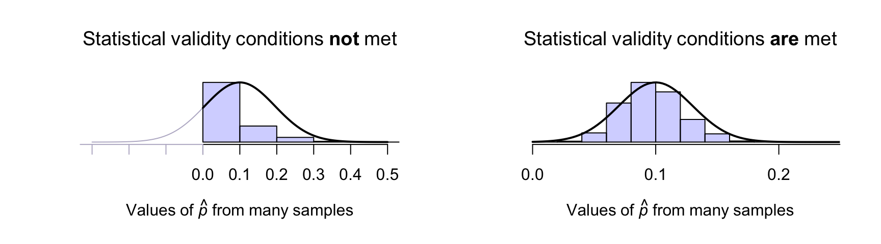
FIGURE 22.6: Two proposed sampling distributions. The sampling distribution from many simulated samples is shown in the histogram; the normal model is shown by the solid lines. Left: when the statistical validity conditions are not met. Right: when the statistical validity conditions are met.
22.8 Example: female coffee drinkers

Kelpin et al. (2018) studied \(360\) female college students in the United States, and found that \(61\) drank coffee daily. The parameter is \(p\), the unknown population proportion of female college students in the United States that drink coffee daily.
The sample size is \(n = 360\), and the sample proportion of daily coffee drinkers is \(\hat{p} = 61/360 = 0.16944\). Of course, the sample proportion varies from sample to sample, so the sample proportion has sampling variation, measured by the standard error: \[ \text{s.e.}(\hat{p}) = \sqrt{ \frac{ 0.16944 \times (1 - 0.16944)}{360}} = 0.01977. \] An approximate \(95\)% CI is \(0.16944 \pm (2 \times 0.01977)\), or \(0.16944 \pm 0.03954\) (i.e., the margin of error is \(0.03954\)). Equivalently, the approximate \(95\)% CI is from \(0.130\) to \(0.209\), after rounding appropriately. We write:
The sample proportion of female US college students who drink coffee daily is \(\hat{p} = 0.169\) (\(n = 360\)), with an approximate \(95\)% CI from \(0.130\) to \(0.209\).
That is, values for \(p\) that may have led to this value of \(\hat{p} = 0.1694\) are between \(0.130\) and \(0.209\) with \(95\)% confidence. (This CI may or may not contain the true proportion \(p\).) This CI is statistically valid, since \(61\) in the sample drink coffee, and \(299\) do not (and both exceed five).
Many decimal places are used in the working, but final answers are rounded.
22.9 Chapter summary
To compute a confidence interval (CI) for a proportion, compute the sample proportion, \(\hat{p}\), and identify the sample size \(n\) used to compute \(\hat{p}\). Then compute the standard error, which quantifies how much the value of \(\hat{p}\) varies across all possible samples: \[ \text{s.e.}(\hat{p}) = \sqrt{\frac{ \hat{p} \times (1-\hat{p})}{n}}. \] The margin of error is (multiplier\({}\times{}\)standard error), where the multiplier is \(2\) for an approximate \(95\)% CI (from the \(68\)--\(95\)--\(99.7\) rule). Then the CI is: \[ \hat{p} \pm \left( \text{multiplier}\times\text{standard error} \right). \] The statistical validity conditions should also be checked.
You must use proportions in these formulas, not percentages; that is, use values between \(0\) and \(1\) (like \(0.169\) rather than \(16.9\)%).
22.10 Quick review questions
Are the following statements true or false?
- \(p\) is a parameter.
- The value of \(p\) will vary from sample to sample.
- The standard error refers to the sampling variation in \(p\).
- Suppose \(n = 50\) and \(\hat{p} = 0.4\); then the standard error of \(\hat{p}\) is \(0.06928\).
22.11 Exercises
Answers to odd-numbered exercises are given at the end of the book.
Exercise 22.1 G.-W. Lee et al. (2016) found that \(708\) of \(864\) patients examined with hiccups were male in their sample.
- Compute the sample proportion of people with hiccups who are male.
- Find an approximate \(95\)% CI for the proportion of people with hiccups who are male.
- Check if the statistical validity conditions are met or not.
- Draw a sketch of how the sample proportion varies for samples of size \(864\).
Exercise 22.2 Lord, Cui, and Kelly (2009) studied how paramedics administer pain medication, and found that \(791\) of patients reporting pain did not receive pain relief, out of \(1\,766\) patients in the study who initially reported pain.
- Compute the sample proportion of patients who did not receive pain medication.
- Find an approximate \(95\)% CI for the proportion of patients who did not receive pain medication.
- Check if the statistical validity conditions are met or not.
- Draw a sketch of how the sample proportion varies for samples of size \(1\,766\).
Exercise 22.3 For an approximate \(95\)% CI, the multiplier (from the \(68\)--\(95\)--\(99.7\) rule) is \(2\). Use Appendix B.1 to find the exact value for the multiplier.
Exercise 22.4 Use Appendix B.1 to find the exact value for the multiplier to create a \(99\)% CI.
Exercise 22.5 Mann and Blotnicky (2017) studied the eating habits of university students in Canada. They found that \(8\) students out of \(154\) met the recommendation for eating a sufficient number of servings of grains each day.
- Find an approximate \(95\)% CI for the population proportion of Canadian students that meet the recommendation for eating a sufficient number of servings of grains each day.
- Check if the statistical validity conditions are met or not.
- Draw a sketch of how the sample proportion varies for samples of size \(154\).
- Would these results be likely to apply to US university students? Explain.
Exercise 22.6 C. E. Dexter et al. (2018) found that \(18\) of the \(n = 51\) koalas studied in a certain area over \(30\) months had crossed at least one road during that time. The parameter is \(p\), the unknown population proportion of koalas that had crossed at least one road over the \(30\) months.
- Find an approximate \(95\)% CI for the proportion of koalas that had crossed the road at least once in the \(30\) months.
- Check if the statistical validity conditions are met or not.
- Draw a sketch of how the sample proportion varies for samples of size \(51\).
Exercise 22.7 Sutherland et al. (2012) studied salt intake in the United Kingdom, and found that \(2\,182\) out of the \(6\,882\) people sampled in 2007 'generally added salt at the table'. Find an approximate \(95\)% CI for the population proportion of Britons that generally add salt at the table.
Exercise 22.8 A study of turbine failures (Myers, Montgomery, and Vining 2002; Nelson 1982) ran \(42\) turbines for around \(3\,000\,\text{h}\), and found that nine developed fissures (small cracks). Find a \(95\)% CI for the true proportion of turbines that would develop fissures after \(3\,000\,\text{h}\) of use. Are the statistical validity conditions satisfied?
The study also ran \(39\) turbines for around \(400\,\text{h}\), and found that zero developed fissures. Find a \(95\)% CI for the true proportion of turbines that would develop fissures after \(400\,\text{h}\) of use. Are the statistical validity conditions satisfied?
Exercise 22.9 Hammond, Reid, and Zukowski (2018) studied young Canadians aged \(12\)--\(24\), and found \(365\) of the \(1\,516\) respondents reported sleeping difficulties after consuming energy drinks. Find a \(95\)% CI for the true proportion of young Canadians who experience sleeping difficulties after consuming energy drinks. Are the statistical validity conditions satisfied?
Exercise 22.10 McLaughlin (2010) studied the proportion of alcohol-associated calls to the ambulance service over four years in a midwestern American town. Of the \(1\,014\) calls received over the four years, \(500\) were received on the weekend (Saturday and Sunday). Find an approximate \(95\)% CI for the true proportion of alcohol-related calls that occur on the weekend.
Exercise 22.11 Oca et al. (2023) used three different AI chatbots to produce recommendations for ophthalmologist in the \(20\) largest cities in the USA. ChatGPT made \(44\) recommendations, of which \(14\) were female. Find an approximate \(95\)% CI for the true proportion of female ophthalmologists recommended in those \(20\) cities.
Exercise 22.12 ChatGPT was launched in 2022. V. R. Lee et al. (2024) studied the impact on cheating for Californian high-school students in 2023. Students were asked to respond to this question (among many others):
In the past month, how often have you used an Artificial Intelligence or digital device (e.g. ChatGPT, smart phone) as an unauthorised aid during an assessment, school assignment, or homework.
Options were 'Never', 'Once', '\(2\) to \(3\) times' and '\(4\) or more times'.
In private high schools, \(13\) of \(202\) students reported using AI in this manner at least once. Find an approximate \(95\)% CI for the true proportion of students using ChaptGPT in this manner in 2023.
Exercise 22.13 [Dataset: HatSunglasses]
B. Dexter et al. (2019) recorded the number of people at the foot of the Goodwill Bridge, Brisbane, who wore hats between \(11\):\(30\)am to \(12\):\(30\)pm.
Of the \(752\) people observed, \(101\) wore hats.
Find an approximate \(95\)% CI for the true proportion of people wearing hats at this time at the foot of the Goodwill Bridge.
Exercise 22.14 [Dataset: HatSunglasses]
B. Dexter et al. (2019) recorded the number of people at the foot of the Goodwill Bridge, Brisbane, who wore sunglasses between \(11\):\(30\)am to \(12\):\(30\)pm.
Of the \(752\) people observed, \(249\) wore sunglasses.
Find an approximate \(95\)% CI for the true proportion of people wearing sunglasses at this time at the foot of the Goodwill Bridge.