7 Internal validity in experimental studies | Scientific Research and Methodology

7.1 Introduction

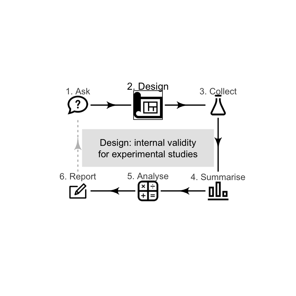
A well-designed study is needed to draw solid conclusions (Def. 6.2): a study with high internal validity (Sect. 6.1) and high external validity (Sect. 5.1). Some research design decisions to maximise internal validity are discussed in this chapter (for experimental studies).

Example 7.1 (Importance of internal validity) Beaman et al. (2013) describe an experiment where free fertilizer was provided to a sample of female farmers in Mali (at the recommended rate, or at half the recommended rate).

The farmers knew they were in the study, so changed their farm management: they employed more hired labour and used more herbicide. Consequently, the yields for all farmers improved, so knowing if the fertilizer dose impacted yield is difficult. The study had poor internal validity.

Specific design strategies for maximising internal validity include:

Managing confounding (Sect. 7.2).
Managing the Hawthorne effect by blinding individuals (Sect. 7.4).
Managing the observer-effect by blinding the researchers (Sect. 7.5).
Managing the placebo effect by using objective measures and controls (Sect. 7.6).
Managing the carry-over effect by using washouts (Sect. 7.7).

Not all of these strategies will be relevant to every study. This chapter discusses experimental studies; the next chapter considers design strategies for observational studies.

For this chapter, consider this relational RQ (based on Bird et al. (2008)) with an intervention:

Among Australians, is the average faecal weight the same for people eating provided food made from wholegrain Himalaya 292 compared to eating provided food made from refined cereal?

7.2 Managing confounding

Suppose that the researchers for the Himalaya 292 study created two groups:

Group A: women recruited at a female-only gym.
Group B: men recruited at a local nursing home.

The researchers then gave Himalaya 292 to Group A, and the refined cereal to Group B. If a difference in faecal weight was detected between the two groups, the difference may due to:

the different diets (the explanatory variable) for each group;
the different sexes in each groups (Group A was all women; Group B was all men);
the different ages in each group (Group A is likely to be younger on average than those in Group B);
the different overall health in each group (Group A would generally be healthier than those in Group B).

Any difference in faecal weight detected between the two groups may not be because of the diets (Table 7.1): the study has very poor internal validity, due to poor research design.

Sex, age and overall health are confounding variables (Def. 6.5). For example, the age of the subject may be related to faecal weight (older people tend to eat less, and eat differently, than younger people), and the research design means that older people are more likely to be consuming the refined cereal. This is an extreme case of confounding (Fig. 7.1); usually, confounding is more subtle (and more difficult to detect) than in this example.

TABLE 7.1: Comparing Groups A and B: An extreme example of confounding

Group A		Group B
Women	Sex	Men
Younger (in general)	Age	Older (in general)
Himalaya 292	Cereal	Refined
Very fit (in general)	Fitness	Less fit (in general)

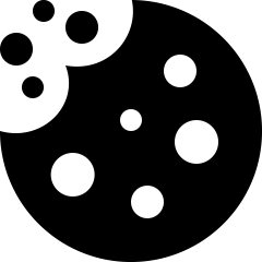
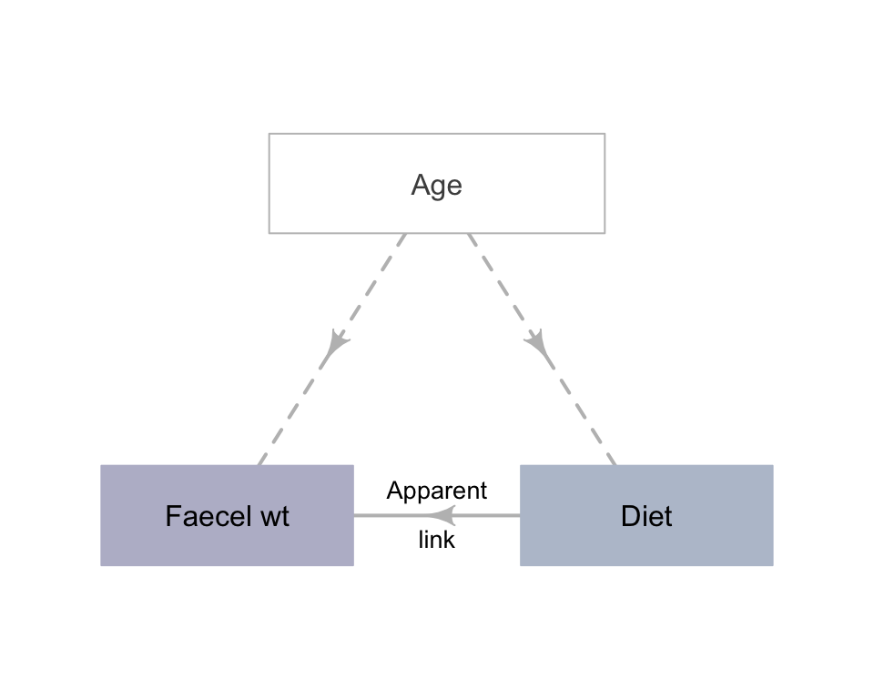
FIGURE 7.1: An extreme example of confounding

The groups being compared should be as similar as possible, apart from the difference being studied.

Confounding can be managed by:

Restricting the study to a certain group, by keeping some variables approximately constant. These variables are called control variables. If possible, a reason for this restriction should be given.
Blocking. Units of analysis are arranged into different groups contining individuals that are similar to one another (see Sect. 34.1 for an example).

Definition 7.1 (Blocking) Blocking occurs when units of analysis are arranged in separate groups of similar units (called blocks).

Analysing using special methods (beyond this book), after recording the values of potential confounding variables. Because of this, recording all potential extraneous variables is important. Most studies involving people record the participants' age and sex, as these two variables are common confounders. Once a sample is obtained, recording this extra information usually requires little extra effort.
Randomly allocating individuals to the comparison groups. Random allocation should ensure that potential confounding variables are approximately evenly spread between the comparison groups. This is true for potential confounders that have been identified (such as age), and also for variables that may not have even been considered as confounders, or are hard to measure or observe (such as genetic conditions).

Record all the extraneous variables likely to be important for understanding the data. This may include information about the individuals in the study, and the circumstances of the individuals in the study.

Multiple approaches can be used, such as randomly allocating individuals to groups, and recording other variables that can be managed through analysis.

Restricting and blocking are useful if one or two variables are known, or thought likely, to cause confounding. Analysing requires recording all the variables suspected of being confounders. Randomly allocating is superior when possible, because the chance of confounding is reduced for variables not even suspected as being confounders.

Common to many of these methods is to ensure that any potential confounding variables are recorded (Sect. 7.9), to ensure no lurking variables exist that may compromise the results.

Example 7.2 (Managing confounding) For the Himalaya study, different methods can be used to manage confounding due to age.

The study could be restricted to only study people under \(30\). Age would be the control variable.

Blocking could be used by finding similar pairs of subjects (e.g., pairs of subjects of the same sex, with similar age and weight). Then, one of each pair is given the refined cereal diet, and one given the Himalaya 292 diet. The differences in faecal weight for each pair can be analysed using special methods (see Chap. 34 for example).

Information about the individuals could be recorded, such as age and pre-study weight. Information about the circumstances of the individuals could also be recorded, such as the suburb where they live. Then, special methods of analysis could be used to analyse the data.

Participants could be randomly allocated into one of two groups, so both groups would have a similar spreads of ages (and other potential confounders). Then groups could be randomly allocated to receive one of the diets (Fig. 7.2).

In the Himalaya 292 study, individuals were randomly allocated randomly to the diets (p. 1033).

FIGURE 7.2: Random allocation can occur in two places for the Himalaya study

An experiment to study the effect of using ginko to enhance memory (Solomon et al. 2002) compared two groups: one using ginko (\(n = 111\)), and one using a fake, non-active supplement (\(n = 108\)). The authors randomly allocated participants to each group, then compared the two groups to ensure that no obvious differences initially existed between the groups that might explain differences in the response variable (Table 7.2).

Two groups are similar in terms of age, education and gender distribution. Any difference in outcome between the groups is probably due to the treatment.

TABLE 7.2: Comparing the two groups in the ginko-memory study
Characteristic	Group A (Ginko)	Group B (Fake)
Average age (in years)	68.7	69.9
Men (number; percentage)	46 (41%)	45 (42%)
Average years of education	14.4	14.0

Researchers explored the use of dominant and non-dominant hands for chest compression in student paramedics using an experimental study (Cross et al. 2019). Students were randomly divided into two groups: DHOS (dominant hand on chest) and NDHOC (non-dominant hand on chest). The two groups were then compared:

Demographic	All participants (\(n = 75\))	DHOC (\(n = 37\))	NDHOC (\(n = 38\))
Average age (years)	\(23.4\)	\(22.5\)	\(24.3\)
Gender: percentage Female	\(51\)%	\(53\)%	\(47\)%

The two groups appear to be very similar in terms of average age of participants, and the percentage of female participants. If differences are observed in the study between the DHOC and NDHOC groups, it is probably due to the treatment. The study should have reasonable internal validity.

Example 7.3 (Analysis to manage confounding) An experimental study (Schröder et al. 2015) compared nitrogen (N) and phosphorus (P) concentrations in maize, for evenly-injected liquid manure and band-injected liquid manure. As potential confounding variables, the researchers also recorded the average temperature and the precipitation (between May 1 and September 30) at each site.

Individuals may be randomly allocated into groups (in true experiments). In addition, groups may be randomly allocated to receive treatments (in true and quasi-experiments).

7.3 Random allocation vs random sampling

Random sampling and random allocation are different concepts (Fig. 7.3), with different purposes, but are often confused:

Random sampling impacts external validity. Its purpose is finding individuals to study.
Random allocation helps eliminate confounding issues, by distributing possible confounders across treatment groups. Random allocation impacts internal validity. Its purpose is allocating treatments to individuals.

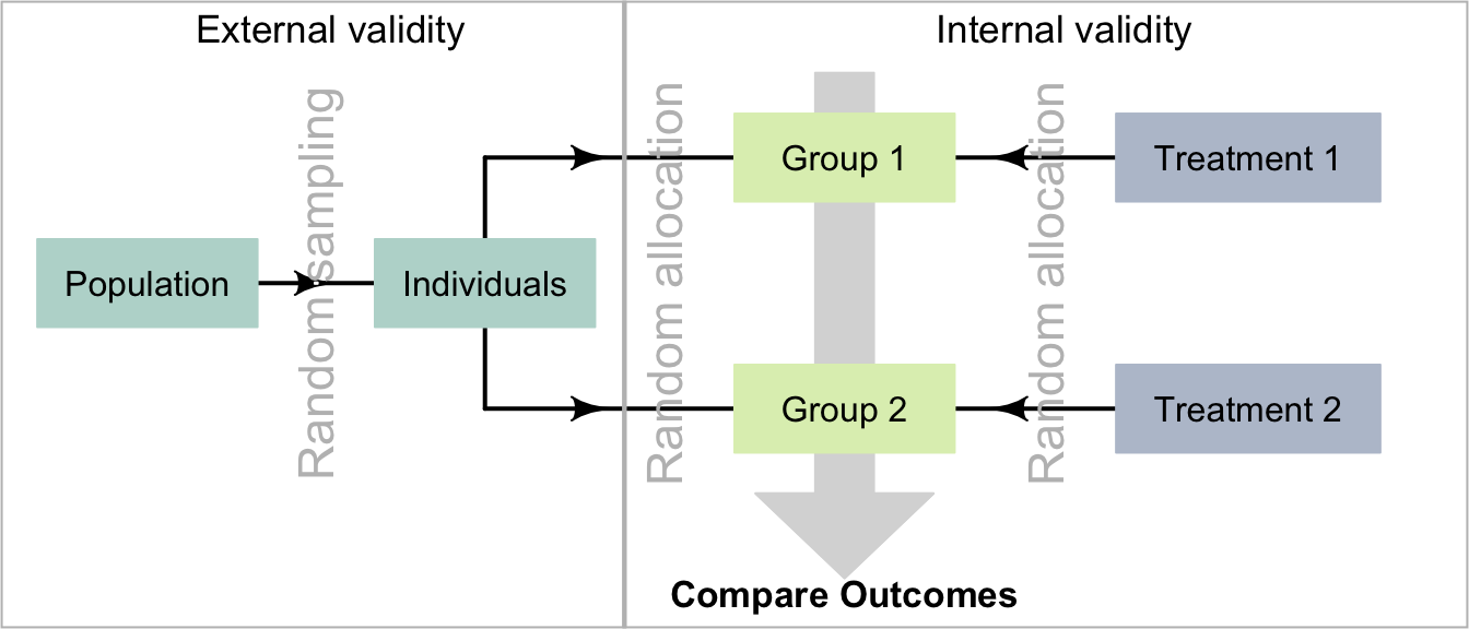
FIGURE 7.3: Comparing random allocation and random sampling

7.4 Hawthorne effect and blinding individuals

Suppose patients in the Himalaya 292 study were being watched (or waited for) while defecating. Could this lead to a misleading conclusion?

People, and perhaps animals, may behave differently if they know (or think) they are being watched, which could compromise the internal validity of the study. This is called the Hawthorne effect.

Definition 7.2 (Hawthorne effect) The Hawthorne effect is the tendency of individuals to change their behaviour if they know (or think) they are being observed.

Example 7.4 (Hawthorne effect) People are more health-conscious if they know they will be examined regularly. For example, a study aiming to increase fruit and vegetable intake in young adults (Clark et al. 2019) noted that the observed increases in intake 'could be explained by the Hawthorne effect' as they 'know they are being observed...'. (p. 96).

The impact of the Hawthorne effect can be minimized by blinding the individuals in the experiment, so that:

the individuals do not know that they are participating in a study; and/or
the individuals do not know the aims of the study; and/or
the individuals do not know which treatment they are receiving in the study.

Blinding people to knowing they are involved in a study is often difficult, as ethics often requires informed consent (Sect. 4.2).

Example 7.5 (Hawthorne effect) The Himalaya 292 article reports that (p. 1033):

The study was explained fully to the subjects, both verbally and in writing, and each gave their written, informed consent...

That is, the subjects knew they were in a study, and knew the aims of the study, so the Hawthorne effect may influence the results in this study. However, the subjects did not know which diet they were given

Example 7.6 (Hawthorne effect) Lorenz et al. (2019) compared the efficacy of a new type of toothpaste. Participants were given either a new or an existing toothpaste formulation, and evaluations of plaque remaining on the teeth were taken. Both groups recorded a reduced amount of plaque.

The reason was the Hawthorne effect: since all participants knew they were being assessed after brushing, they brushed better than usual.

7.5 Observer effect and blinding researchers

Suppose the researchers assessing the study outcomes knew the diet allocated to each patient. Could this lead to a misleading conclusion?

Perhaps surprisingly, researchers' expectations or hopes for how the new diet will perform may unconsciously influence how the researchers interact with the individuals, and so perhaps (unconsciously) influence the behaviour of the individuals in the study. This is called observer effect. (In experiments, it is sometimes called the experimenter effect.) This could compromise the internally validity of the study.

Definition 7.3 (Observer effect) The observer effect occurs when the researchers unconsciously change their behaviour to conform to expectations because they know what values of the explanatory variable apply to the individuals. This may then cause the individuals to change their behaviour or reporting also.

The impact of the observer effect can be minimized by blinding the researchers, so that they do not know which treatments the individuals are receiving. The researchers giving the treatment and the researchers evaluating the treatment can both be blinded, by using a third party. For example, the researchers may give an assistant two drugs, labelled A and B. The assistant administers the drug and evaluates the participants' response to the treatments. Later, the assistant tells the researchers whether Drug A or Drug B performed better, but only the researchers know which drugs the labels A and B refer to (Fig. 7.4).

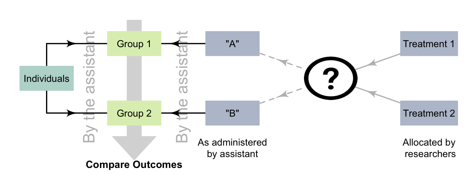
FIGURE 7.4: Using a third party to avoid the observer effect

Example 7.7 (Observer effect) In a study (Seo et al. 2020) that examined the impact of an injection to alleviate post-operative umbilical pain, the authors stated (p. 392):

...the postoperative pain scores were gathered by a nurse practitioner who was blinded to the usage of bupivacaine to avoid observer-expectancy bias [i.e., the observer effect].

The observer effect does not just apply to situations with people as individuals.

Example 7.8 (Observer effect) 'Clever Hans' was a horse that seemed to perform simple mental arithmetic. By using an experiment where the people interacting with the horse were blinded, Carl Stumpf realised that the horse was responding to involuntary (and unconscious) cues from the trainer.

The same effect has been observed in narcotic sniffer dogs (Bambauer 2012), who may respond to their handlers' unconscious cues.

The observer effect is when the researcher unconsciously influence the individuals, and are not aware it is occurring. Intentionally influencing the individuals is fraud.

7.6 Placebo effect, controls and blinding

To know whether the Himalaya diet changed faecal weight, the researchers compared the outcome for people on the Himalaya diet to the outcome for people on a refined-cereal diet. The people on the refined-cereal diet acted as the control group (Sect. 2.7). The refined cereal acted as a benchmark; like a placebo.

Perhaps surprisingly, individuals in a study may report effects of a treatment, even if they have not received an active treatment. This could compromise the internally validity of the study. This is called the placebo effect, which generally only impacts people as individuals.

Definition 7.4 (Placebo effect) The placebo effect occurs when individuals report perceived or actual effects, despite not receiving an active treatment.

To manage the placebo effect, researchers should record objective data rather than patient-reported outcomes when possible (Enck et al. 2013). In addition, blinding the individuals and the researchers may help manage the placebo effect, as then the individuals cannot know which group they are in.

Example 7.9 (Placebo effect) Three active pain relievers were compared to different-coloured placebo (Huskisson 1974) in \(22\) patients. The most pain relief was experienced by those taking red placebos (Fig. 7.5), who experienced even more pain relief than those given true pain relievers. Note that the outcome is subjective: a patient-reported outcome.

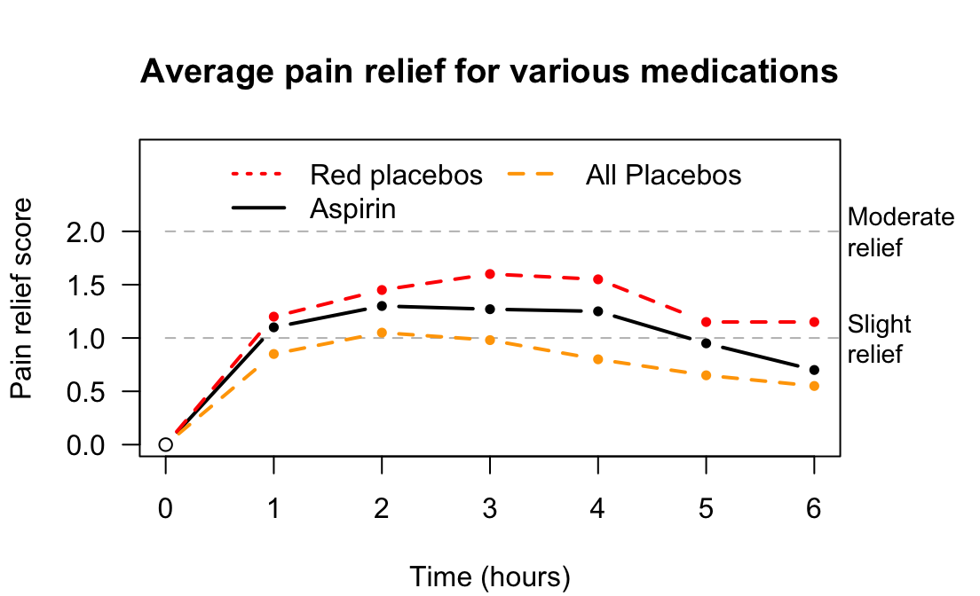
FIGURE 7.5: Pain relief, for various pain relief medicine and placebos

Example 7.10 (Placebo effect) In the Himalaya study, the individuals 'were not told the identity of the test cereal in the foods provided' (Bird et al. (2008), p. 1033). The subjects were blinded to the diet they were exposed to. However, some may think they are on the refined cereal or Himalaya diet, and respond accordingly (perhaps unconsciously). The use of the refined cereal was acting as a control. Researchers measured faecal weight, an objective outcome, to minimise the placebo effect.

A study of placebos (Waber et al. 2008) gave half the subjects a placebo, but told them the pill was an expensive (implying 'effective') pain killer. The other half were also given a placebo, but were told the pill was a discount (implying 'less effective') pain killer. About \(85\)% of participants in the first group reported a pain reduction, yet only \(61\)% in the second group reported a pain reduction. Remember: both groups actually received a placebo! Again, 'pain relief' is subjective.

7.7 Carry-over effect and washouts

In the Himalaya study, the diet is a between-individuals comparison: one group of patients is given the refined cereal diet (the control), and a different group of people was given Himalaya 292. The study also used a within-individuals comparison: each person in the study was actually placed on both diets at different times.

Suppose all patients spent four weeks on the Himalaya 292 diet, then the next four weeks on the refined cereal diet. Potentially, the first diet could still be impacting the subjects' faecal weight for a little while after stopping the first diet. This could compromise the internally validity of the study. This is an example of the carry-over effect: when the influence of one treatment carries over to influence the next treatment. The carry-over effect is only a concern for within-individuals comparisons.

Definition 7.5 (Carryover effect) The carry-over effect occurs when the influence of one treatment influences individuals' responses to subsequent treatments.

The impact of the carry-over effect may be minimized by using a washout or similar between treatments. For example, after tasting a food sample, participants may rinse their mouth with water before tasting another food sample. For the Himalaya study, between using the special diets, the participants could spend two weeks on their usual (before-study) diet. This is called a washout period.

Example 7.11 (Carry-over effect) In the Himalaya study, 'there was no washout period' (Bird et al. (2008), p. 1033) since the response variable was only recorded after individuals spent four weeks on each diet. Since faecal weight was not measured until the end of this four weeks, the effect of the diet change would be minimal.

Example 7.12 (Carry-over effect) An engineering study (Miller and Boyle 2019) examined drivers' exposure to lane-keeping systems on their driving performance. Subjects were exposed to a driving simulation that used a lane-keeping system, and then to a driving simulation without using a lane-keeping system. The researchers found that driving performance was impacted when drivers moved from a simulation with a lane-keeping system to one without a lane-keeping system.

In Jaskiewicz et al. (2020), student paramedics performed chest compression in real-life (RL), and also using virtual reality (VR). A relaxation percentage of about \(50\)% is ideal.

When used by itself, the VR method produced an average relaxation percentage of \(45.5\)%. However, when the RL method was used first, and then followed by the VR method, the average VR relaxation method percentage was \(74.7\)%.

The response of the individuals was different depending on whether the RL method was used first. This is an example of the carry-over effect.

Sometimes, when relevant, researchers can randomly allocate the order in which the treatments (i.e., the diets) are used (a cross-over study). That is, some participants start by spending four weeks on the Himalaya 292 diet, then four weeks on the refined cereal diet; meanwhile, other participants start by spending four weeks on the refined cereal diet, then four weeks on the Himalaya 292 diet.

Example 7.13 (Carry-over effect) In the Himalaya study, the 'subjects were allocated randomly to [...] dietary treatments' (Bird et al. (2008), p. 1033). Subjects were randomly allocated to begin the study on either the Himalaya 292 diet or the refined cereal diet.

Example 7.14 (Washout periods) R. D. MacDonald et al. (2006) required paramedics to conduct eight different tasks (such as electrical defibrillation and intravenous cannulation). Each of the \(16\) paramedics began the series of tasks at a random task, to mitigate the carry-over effect. A washout period between tasks was also used.

7.8 Describing blinding

Blinding occurs when those involved in the study do not know information about the study. Individuals in the study may be blinded to

whether they are involved in a study;
the aims of the study in which they are participants; and/or
which comparison group they are in.

The researchers and the analysts can be blinded to which comparison groups apply to the individuals.

When blinding is used in as many ways as possible, the internal validity of the study is increased and bias reduced. However, when people are the individuals, ethics requirements may mean that they need to know they are in a study (especially if the study is experimental), and the purpose of the study.

If only the individuals are blinded to the comparison groups, the study is called single blind. If both the researchers and participants are blinded to the comparison groups, the study is called double blind. If the researchers, participants and the analyst are blinded to the comparison groups, the study is called triple blind. Rather than using these terms, explicitly stating who or what is blinded is clearer.

Why might it be necessary to blind the analyst to the treatments used?

Blinding should be considered in all studies when possible (it is not always possible). Blinding participants does not just apply to people; it also may apply to animals (Example 7.8).

Example 7.15 (Double-blinding) Bulte et al. (2014) compared yields from modern and traditional cowpea crops in Tanzania. The two seed types ('traditional' and 'modern') were made similar in appearance so the farmers were blinded. The seed type would eventually become obvious as the crop grew, but 'key inputs were already provided' by then (p. 817).

7.9 Recording extraneous variables

One way to design a quality study is to record information about many extraneous variables. Various reasons for doing this have been given:

To evaluate external validity to determine if the sample is representative of the population (Sect. 5.10), by comparing the sample and population.
To improve internal validity, by helping to manage confounding:
- by using special methods of analysis (Sect. 6.5).
- by avoiding lurking variables (Sect. 6.5).
- by determining if the groups being compared are similar (Sect. 7.2).
- by using the information in analysis (Sect. 7.2).

Record the values of all extraneous variables that may be important in the study!

7.10 Chapter summary

Designing effective experimental studies (Fig. 7.6) requires researchers to manage or minimise confounding where possible, by restricting the study to certain groups; blocking individuals into similar groups; through special analysis methods; and/or through random allocation of the units of analysis.

Well-designed experimental studies also try to manage the Hawthorne effect (e.g., by blinding participants); the observer effect (e.g., by blinding the researchers); the placebo effect (e.g., by using controls, and using objective outcomes); and the carry-over effect (e.g., by using a washout, or randomly allocating the treatment order). This ensures that the results and conclusions from our studies are correctly interpreted.

The following short video may help explain some of these concepts:

Often, however, not all of these strategies can always be used. For instance, people often know they are involved in an experimental study, so the Hawthorne effect may impact conclusions. In these cases, the possible impacts should be minimized as far as possible, and then the likely impact on the conclusions discussed. The impact of these issues are often reported as limitations in a journal article (Chap. 9).

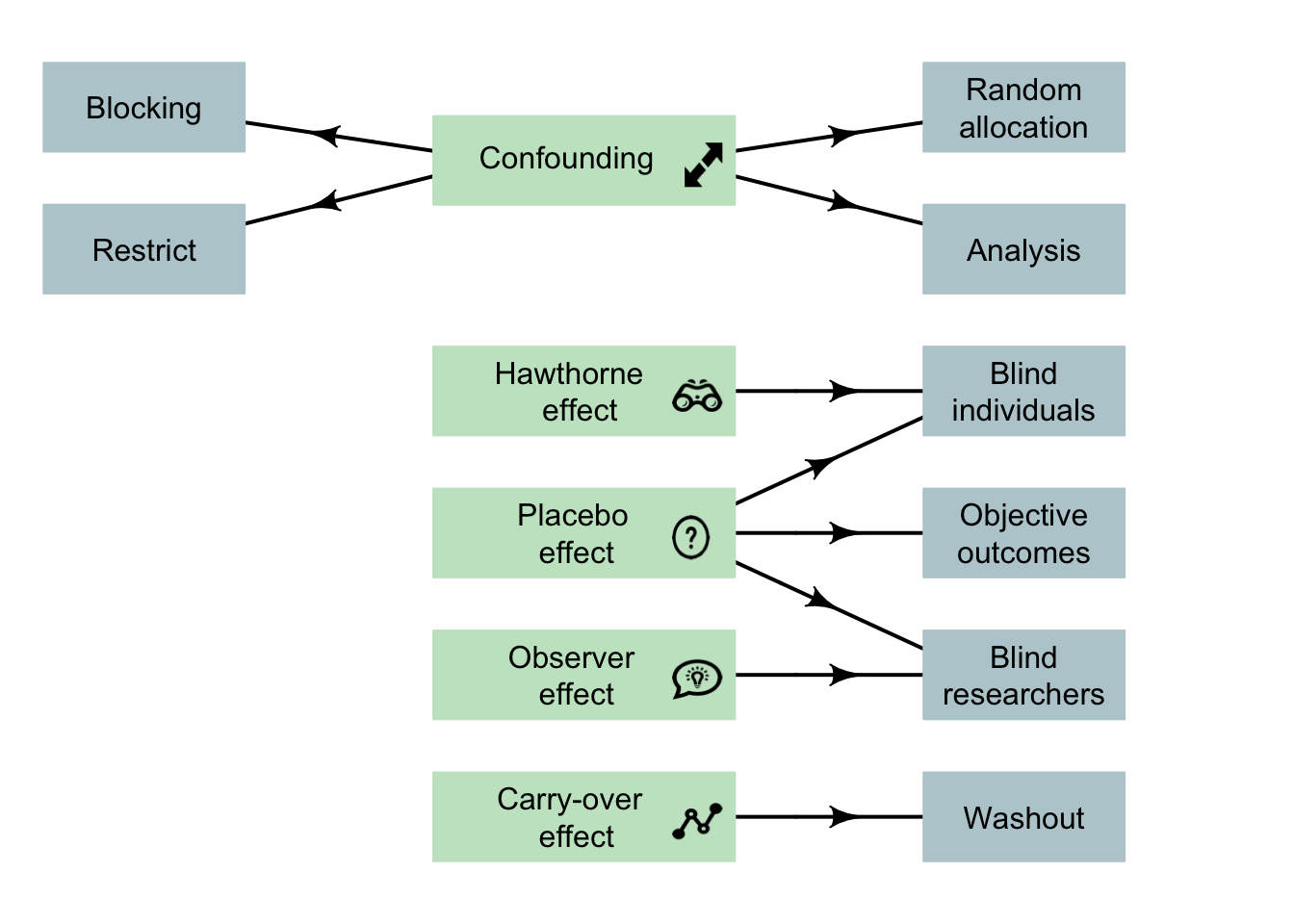
Design considerations for experimental studies. Note: lurking variables become confounding variables when recorded in the study, and so can be managed. The arrows indicate the main design strategy to (perhaps partially) manage the indicated potential bias. Not all strategies are possible for every study.

FIGURE 7.6: Design considerations for experimental studies. Note: lurking variables become confounding variables when recorded in the study, and so can be managed. The arrows indicate the main design strategy to (perhaps partially) manage the indicated potential bias. Not all strategies are possible for every study.

Example 7.16 (Research design) Cross et al. (2019) (p. 3) comparing chest compressions by student paramedics using dominant and non-dominant hands:

...participants were allocated randomly to one of two groups: 'dominant hand on chest' or 'non-dominant hand on chest'. Group allocation was determined by a computer-generated randomisation schedule...

The participants were blinded to the purpose of the study, but not to which group they were allocated. The analyst was also blinded to the group allocations. This study used many good design features.

7.11 Quick review questions

7.12 Exercises

Answers to odd-numbered exercises are available in App. E.

Exercise 7.1 Are the following statements true or false?

Experimental studies must use random samples.
An experimental study must blind the researchers.
An experimental study must blind the participants.
Experimental studies must use a control group.
In experimental studies, the treatments must be allocated by the researchers.

Exercise 7.2 Which of the following can be used to improve internal validity in experiments?

Blinding the individuals.
Using a control group.
Using special methods of analysis.
Randomly allocating treatments to groups.
Blinding the researchers.
Using random samples.

Exercise 7.3

Extraneous variables are variables that are related to the response variable.
Which of the following types of variables are special types of extraneous variables?

Lurking variables
Explanatory variables
Confounding variables

Exercise 7.4 Consider a study comparing the average weight loss for patients who are instructed to do at least \(30\) mins of exercise a day (Group A), to patients who are instructed to do less than \(30\) mins of exercise a day (Group B). Which of the following statements are true?

The extraneous variable is the amount of exercise per day (in hours).
The response variable is the weight loss for each person.
The explanatory variable is whether or not the patient performs at least \(30\) minutes of exercise per day.
The response variable is the average weight loss.
The explanatory variable is the amount of exercise the patient does per day (in hours).
Age is likely to be a lurking variable.
Age is an extraneous variable.
Age is likely to be a confounding variable.
Which (if any) of the following are possible confounding variables?
- The sex of the patients.
- The initial weight of the patients.
- The names of the patients.

Exercise 7.6 A scientist compares the effects of two types of fertiliser on the yield of tomatoes (based on Klanian et al. (2018)). He plants tomato seedlings, and fertilises with Fertiliser I, and later records the yield of tomatoes. He then immediately plants more tomato seedlings in the same field, fertilises with Fertilizer II, and measures the yield of tomatoes.

What potential problems can you identify with the research design?

Exercise 7.7 A scientist is testing whether tap water tastes the same as bottled water in a taste test (based on Teillet et al. (2010)). She provides people with a plastic cup of either bottled or tap water, and she asks them to give a rating of the taste on a scale of \(1\) (terrible) to \(5\) (fantastic).

What potential problems can you identify with the research design?

Exercise 7.8 Consider this RQ (based on Teillet et al. (2010)):

For university students, is the taste of tap water better than the taste of bottled water?

This RQ needs some clarification, but you decide to answer this question using an experiment. How would you manage:

random allocation?
blinding?
double blinding?

finding a control?
finding a random sample?

Exercise 7.9 Skulberg et al. (2004) compared two office-cleaning methods (p. 72):

The participants were randomly allocated to an intervention group or a control group using group level matching by sex, level of irritation symptom index, and allergy status [...] The participants and the field researchers were blinded to the group status of the participants [...] the cleaning was done in the evening after the employees had left the building.

The researchers then compared the change in nasal congestion for the two groups (intervention: 'a comprehensive cleaning of all surfaces'; control: 'only a superficial cleaning'), finding only small differences between the two groups. In the analysis, the researchers incorporated age and sex of the office workers.

How did the researchers manage confounding?
What other design features are evident from the quote?
What is the response variable?
What is the explanatory variable?
What are the extraneous variables?