37 Correlation

So far, you have learnt about the research process, including analysing data using confidence intervals and conducting hypothesis tests. In this chapter, you will learn to:

• conduct hypothesis tests for correlation coefficients.

37.1 Introduction: red deer

So far, RQs about single variables (descriptive RQs) and RQs for comparisons (relational and repeated-measures RQs) have been studied. In this chapter (and the next), the relationship between two quantitative variables is studied (correlational RQs) when that relationship is approximately linear .

Consider the age and the weight of the molars of \(n = 78\) male red-deer (Holgate 1965), as seen in Chap. 16 (and the data in that section). The data comprises two quantitative variables, and the scatterplot is repeated in Fig. 37.1.

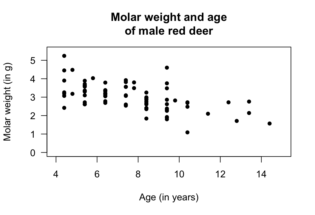
FIGURE 37.1: Molar weight verses age for the red-deer data.

Knowing the age of the deer seems to provide some information about the weight of the molars; that is, a relationship between the variables seems evident. Furthermore, the relationship seems somewhat linear, and in Sect. 16.4.1 the correlation coefficient was found to be \(r = -0.584\).

Only one of the countless possible samples of deer have been studied, and the value of \(r\) will vary from sample to sample. Perhaps the population correlation coefficient \(\rho\) is zero, and only non-zero in the sample due to sampling variation. That is, the sample correlation coefficient is non-zero simply due to sampling variation.

37.2 Statistical hypotheses and the hypothesis test

A correlational RQ can be asked about the relationship between the variables in the population, as measured by the unknown population (Pearson) correlation coefficient:

In the population, is there a linear relationship between the value of \(y\) and the value of \(x\)?

In the context of the red-deer data, the RQ is:

In male red deer, is there a linear relationship between molar weight and age?

This is a two-tailed RQ. More specifically, we could ask a one-tailed research question, since it seems reasonable that teeth get lighter (worn down) as deer age:

In male red deer, does molar weight decrease linearly as age increases?

This is a one-tailed RQ, about the population parameter \(\rho\). Clearly, the sample correlation coefficient \(r\) for the red-deer data is not zero, and the RQ is effectively asking if sampling variation is the reason for this. The null hypotheses is:

• \(H_0\): \(\rho = 0\).

The parameter is \(\rho\), the population correlation coefficient. This null hypothesis is the 'no relationship' position, which proposes that the population correlation coefficient is zero, and the sample correlation coefficient is not zero due to sampling variation. The alternative hypothesis is:

• \(H_1\): \(\rho < 0\) (one-tailed test, based on the RQ).

As usual, initially assume that \(\rho = 0\) (from \(H_0\)), then describe what values of \(r\) could be expected using the sampling distribution, under that assumption, across all possible samples (sampling variation). Then the observed value of \(r\) is compared to the expected values to determine if the value of \(r\) supports or contradicts the assumption.

For a correlation coefficient, the sampling distribution of \(r\) does not have a normal distribution⁸, and software output usually does not provide a standard error, so we will not discuss CIs for the correlation coefficient.

The output (Fig. 37.2) contains the relevant \(P\)-value for the \(t\)-test. The two-tailed \(P\)-value for the test is less than \(0.001\), so the one-tailed \(P\) value will be less than \(0.001/2 = 0.0005\). Very strong evidence exists to support \(H_1\) (that the correlation in the population is less than zero). We write:

The sample presents very strong evidence (one-tailed \(P < 0.0005\)) that the molar weight decreases as the age of the male red deer increases (\(r = -0.584\); \(n = 78\)) in the population.

Notice the three features of writing conclusions again: An answer to the RQ; evidence to support the conclusion ('one-tailed \(P < 0.0005\)'; here no value for the test statistic is given in the output); and some sample summary information ('\(r = -0.584\); \(n = 78\)').

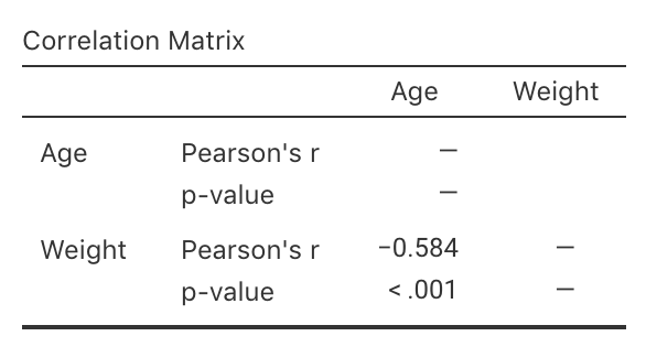
FIGURE 37.2: Software output for the red-deer data.

The evidence suggests that the correlation coefficient is not zero (in the population). However, a non-zero correlation doesn't necessarily mean a strong correlation exists. The correlation may be weak in the population (as estimated by the value of \(r\)), but evidence exists that the correlation is not zero in the population.

That is, the test is about statistical significance, not practical importance.

37.3 Statistical validity conditions

As usual, these results hold under certain conditions. The conditions for which the test is statistically valid are:

1. The relationship is approximately linear (this is necessary for the correlation coefficient to be appropriate).
2. The variation in the response variable is approximately constant for all values of the explanatory variable.
3. The sample size is at least \(25\).

The sample size of \(25\) is a rough figure; some books give other values. The units of analysis are also assumed to be independent (e.g., from a simple random sample).

If the statistical validity conditions are not met, but the relationship is only increasing or only decreasing, other similar options include using a Spearman or Kendall correlation (Conover 2003) or using resampling methods (Efron and Hastie 2021).

Example 37.1 (Statistical validity) For the red-deer data, the scatterplot (Fig. 37.1) shows that the relationship is approximately linear, so using a correlation coefficient is appropriate. For the hypothesis test, the variation in molar weights doesn't seem to be obviously getting larger or smaller for older deer, and the sample size is also greater than \(25\). The test in Sect. 37.2 is statistically valid.

37.4 Example: removal efficiency

In wastewater treatment facilities, air from biofiltration is passed through a membrane and dissolved in water, and is transformed into harmless byproducts. The removal efficiency \(y\) (in %) may depend on the inlet temperature (in \(^\circ\)C; \(x\)). Chitwood and Devinny (2001) asked:

In treating biofiltration wastewater, is the removal efficiency linearly associated with the inlet temperature?

The scatterplot of the \(n= 32\) observations was shown (and described) in Sect. 16.6, and repeated here (Fig. 37.3, left panel); the relationship is approximately linear.

The output (Fig. 37.3, right panel) shows that the sample correlation coefficient is \(r = 0.891\), and so \(R^2 = (0.891)^2 = 79.4\)%. This means that the unexplained variation in removal efficiency reduces by about \(79.4\)% by knowing the inlet temperature.

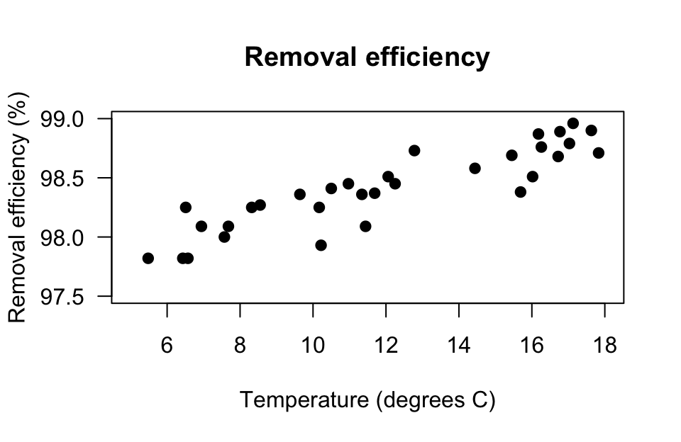
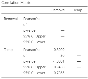
FIGURE 37.3: The relationship between removal efficiency and inlet temperature. Left: scatterplot. Right: software output.

As always, the RQ is about the population parameter \(\rho\), the correlation between the removal efficiency and inlet temperature. To test if a linear relationship exists in the population, write: \[ \text{$H_0$: } \rho = 0\quad\text{and}\quad \text{$H_1$: } \rho \ne 0, \] where \(\rho\) is the population correlation coefficient. The alternative hypothesis is two-tailed (as implied by the RQ). The software output (Fig. 37.3, right panel) shows that \(P < 0.001\). We conclude:

The sample presents very strong evidence (two-tailed \(P < 0.001\)) that removal efficiency depends on the inlet temperature (\(r = 0.891\); \(n = 32\)) in the population.

The relationship is approximately linear, there is no obvious non-constant variation in the removal efficiency, and the sample size is larger than \(25\), so the hypothesis test result is statistically valid.

37.5 Chapter summary

To test a hypothesis about a correlation between two variables, \(\rho\):

• Write the null hypothesis (\(H_0\)) and the alternative hypothesis (\(H_1\)).
• Initially assume the value of \(\rho\) in the null hypothesis to be true (usually zero).
• Software output provides the \(P\)-value for the test, but no test statistic or confidence interval.
• Make a decision, and write a conclusion.
• Check the statistical validity conditions.

The following short video may help explain some of these concepts:

37.6 Quick review questions

A study of Chinese paediatric patients (Wong et al. 2018) studied the relationship between the \(6\)-minute walk distance (\(6\)MWD) and maximum oxygen uptake (VO\(2\)_max) for \(n = 29\) patients. The correlation coefficient is reported as \(r = 0.457\), and the corresponding \(P\)-value as \(P = 0.013\).

1. What is the \(x\)-variable?
   6-minute walk distanceMaximum oxygen uptake
2. True or false: Since the \(P\)-value is small, the correlation is quite strong. TRUE FALSE
3. Is the relationship a positive or negative relationship?
   NegativePositive
4. What is the value of \(R^2\)? (Give the answer to one decimal place, expressed as a percentage.)
5. For statistical validity, what do we need to assume to be true?
   The response variable has a normal distributionThe explanatory variable has a normal distributionThe sample size is larger than 25A linear relationship exists between the variables

37.7 Exercises

Answers to odd-numbered exercises are available in App. E.

Exercise 37.1 LeBlanc et al. (2005) studied \(n = 30\) paramedicine students, and examined the relationship between the amount of stress experienced while performing drug-dose calculations (measured using the State–Trait Anxiety Inventory (STAI)), and length of work experience.

1. Write the hypotheses for testing for a relationship between the STAI score and the length of work experience.
2. The article gives the correlation coefficient as \(r = 0.346\) and \(P = 0.18\). What do you conclude?
3. What must be assumed for the test to be statistically valid?

Exercise 37.2 Einsiedel et al. (2024) studied the relationship between amount of pesticide residue reported on a variety of fresh fruits and vegetables, and various weather measurements. One pesticide studied was the herbicide perchlorate.

1. Write the hypotheses for testing for a relationship between the perchlorate residue and maximum temperature at the growing location.
2. The article gives the correlation coefficient as \(r = -0.059\) and \(P = 0.035\). What do you conclude?
3. Write the hypotheses for testing for a relationship between the perchlorate residue and minimum temperature at the growing location.
4. The article gives the correlation coefficient as \(r = -0.025\) and \(P = 0.365\). What do you conclude?
5. What must be assumed for the tests to be statistically valid?

Exercise 37.3 [Dataset: SDrink] A study examined the time taken to deliver soft drinks to vending machines (Montgomery and Peck 1992) using a sample of size \(n = 25\) (Fig. 37.4, left panel). To perform a test of the correlation coefficient, are the statistical validity conditions met?

Exercise 37.4 [Dataset: Mandible] Royston and Altman (1994) examined the mandible length and gestational age for \(n = 167\) foetuses from the \(12\)th week of gestation onward (Fig. 37.4, right panel). To perform a test of the correlation coefficient, are the statistical validity conditions met?

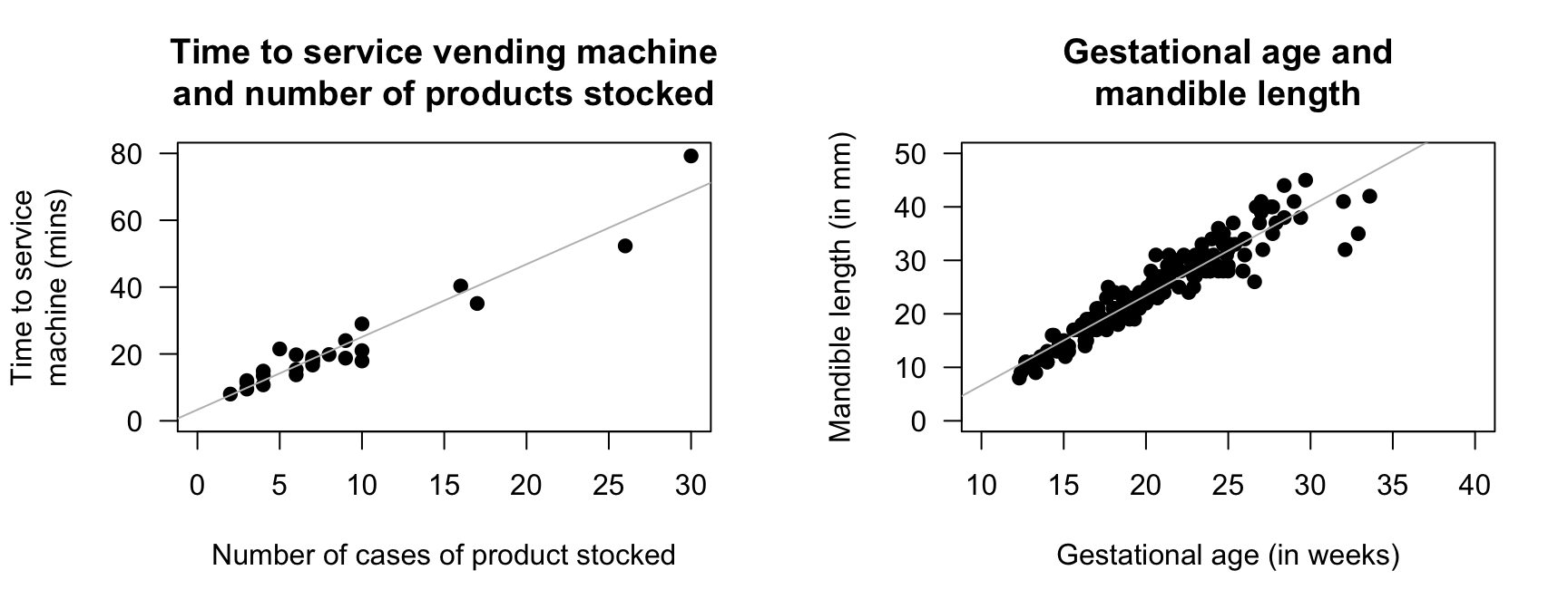
FIGURE 37.4: Two scatterplots. Left: the time taken to deliver soft drinks to vending machines. Right: the relationship between gestational age and mandible length. In both plots, the solid line displays the linear relationship.

Exercise 37.5 [Dataset: Dogs] Quan, Tran, and Chung (2017) studied Phu Quoc Ridgeback dogs (Canis familiaris), and recorded many measurements of the dogs, including body length and body height. The scatterplot displaying the relationship and the software output are shown in Fig. 37.5. In this example, it does not matter which variable is used as \(x\) or \(y\).

1. Describe the relationship.
2. Taller dogs might be expected to be longer. To test this, write the hypotheses.
3. Perform the test, using the output. Write a conclusion.
4. Is the test statistically valid?

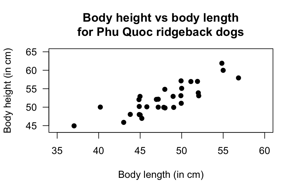
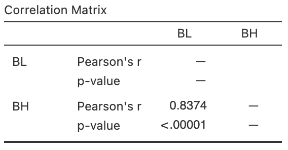
FIGURE 37.5: Phu Quoc ridgeback dogs. Left: a scatterplot of the body height vs body length. Right: software output.

Exercise 37.6 [Dataset: Bitumen] Panda, Das, and Sahoo (2018) made \(n = 42\) observations of hot mix asphalt, and measured the volume of air voids and the bitumen content by weight. The scatterplot displaying the relationship and the software output are shown in Fig. 37.6.

1. Using the plot, estimate the value of \(r\).
2. The value of \(R^2\) is \(99.29\)%. What is the value of \(r\)? (Hint: Be careful!)
3. Would you expect the \(P\)-value testing \(H_0\): \(\rho=0\) to be small or large? Explain.
4. Would the test be statistically valid?

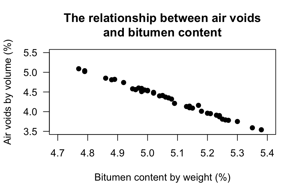
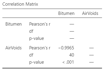
FIGURE 37.6: Bitumen content by weight. Left: a scatterplot. Right: software output.

Exercise 37.7 [Dataset: Punting] Myers (1990) (p. 75) measured the right-leg strengths \(x\) of 13 American football players (using a weight lifting test), and the distance \(y\) they punted a football with their right leg (Fig. 37.7). Use the software output (Fig. 37.7) to answer these questions.

1. Compute the value of \(R^2\), and explain what this means.
2. Perform a hypothesis test to determine if a positive correlation exists between punting distance and right-leg strength.

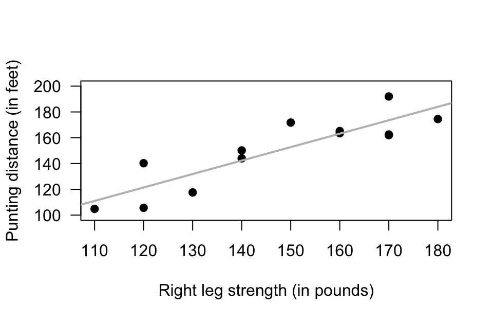
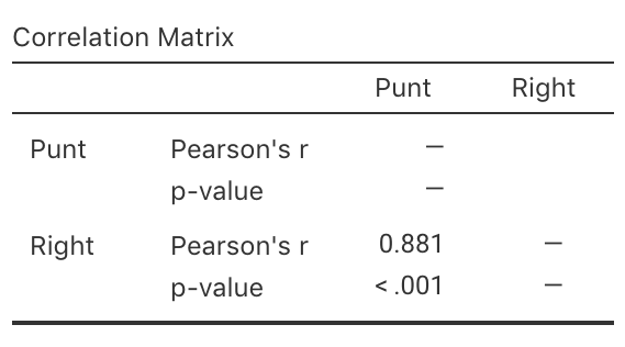
FIGURE 37.7: The punting data. Left: a scatterplot. Right: software output.

Exercise 37.8 [Dataset: Soils] The California Bearing Ratio (CBR) value is used to describe soil sub-grade for flexible pavements (such as in the design of air field runways). Talukdar (2014) examined the relationship between CBR and other properties of soil, including the plasticity index (PI, a measure of the plasticity of the soil). The scatterplot from 16 different soil samples from Assam, India, is shown in Fig. 37.8.

1. Using the plot, take a guess at the value of \(r\).
2. The value of \(R^2\) is \(67.07\)%. What is the value of \(r\)? (Hint: Be careful!)
3. Would you expect the \(P\)-value testing \(H_0\): \(\rho = 0\) to be small or large? Explain.
4. Would the test be statistically valid?

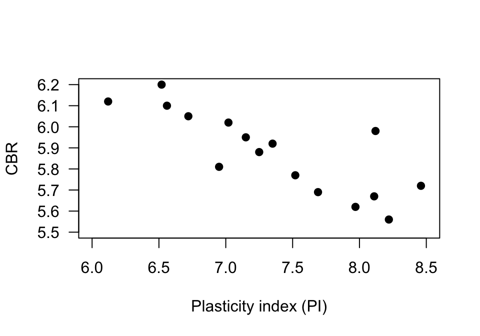
FIGURE 37.8: The relationship between CBR and PI in sixteen soil samples.

Exercise 37.9 [Dataset: Possums] J. L. Williams et al. (2022) studied Leadbeater's possums in the Victorian Central Highlands. They recorded, among other information, the body weight of the possums and their location, including the elevation of the location. A scatterplot of the data and the software output are shown in Fig. 37.9. Using the output (Fig. 37.9), determine the value of \(r\) and \(R^2\). Perform a hypothesis tests, and make a conclusion about the relationship between the chest beating and size of gorillas.

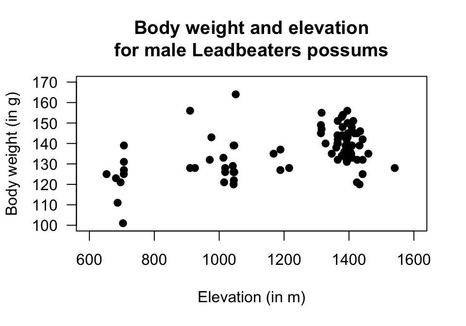
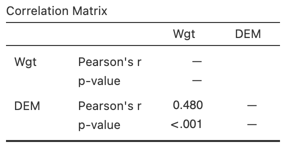
FIGURE 37.9: The relationship between weight of possums and the elevation of their location. Left: scatterplot. Right: software output.

Exercise 37.10 [Dataset: Gorillas] (These data were also seen in Exercise 16.9.) Wright et al. (2021) examined \(25\) gorillas and recorded information about their chest-beating rates and their size (measured by the breadth of the gorillas' backs). The relationship is shown in a scatterplot in Fig. 37.10. Using the software output (Fig. 37.10), determine the value of \(r\) and \(R^2\). Perform a hypothesis tests, and make a conclusion about the relationship between the chest beating and size of gorillas.

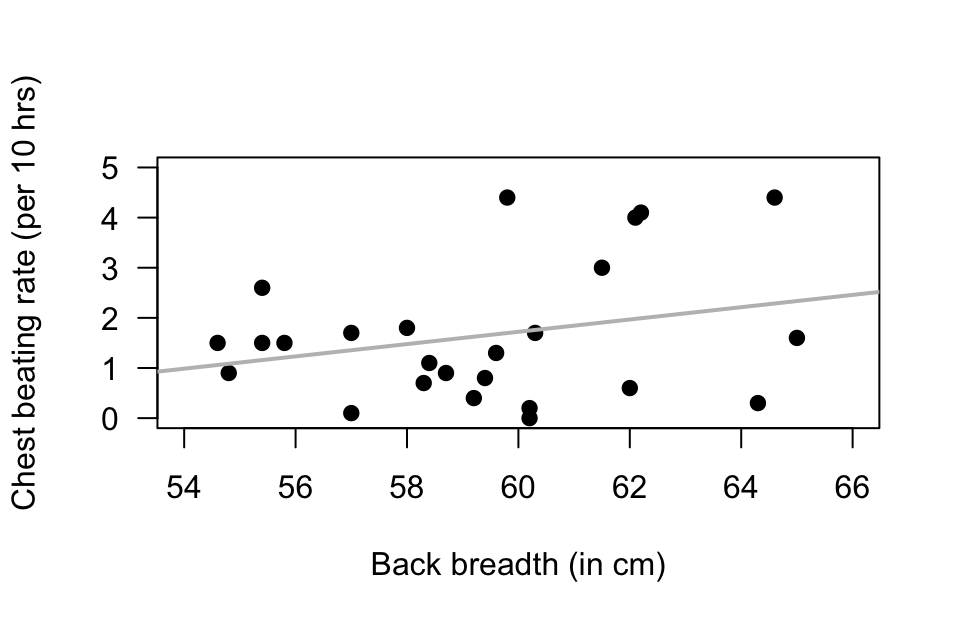
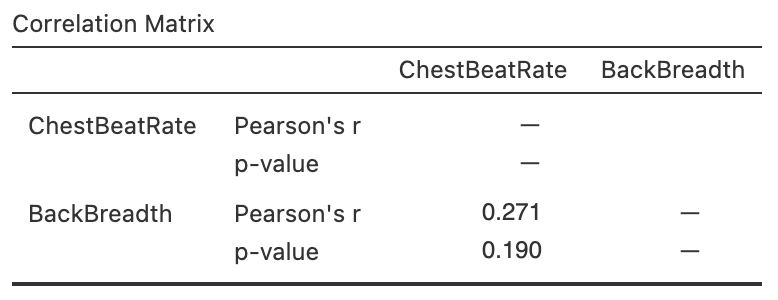
FIGURE 37.10: The punting data. Left: a scatterplot. Right: software output.

Exercise 37.11 [Dataset: Jeans] Diehm and Thomas (2018) recorded data on the size of pockets in men's and women's jeans. This exercise considers the correlation between the maximum widths and maximum heights of front pockets.

1. The correlation in all jeans is \(r = 0.38\); the \(P\)-value for a hypothesis test is \(P = 0.00051\). What does this mean?
2. If only men's jeans are studied, the correlation is \(r = -0.09\) (note: negative value), with \(P = 0.59\). What does this mean?
3. If only women's jeans are studied, the correlation is \(r = 0.14\), with \(P = 0.38\). What does this mean?
4. From the last three questions, how would you describe the relationship between the maximum widths and maximum heights of the front pockets of jeans? (Figure 37.11 may help.)

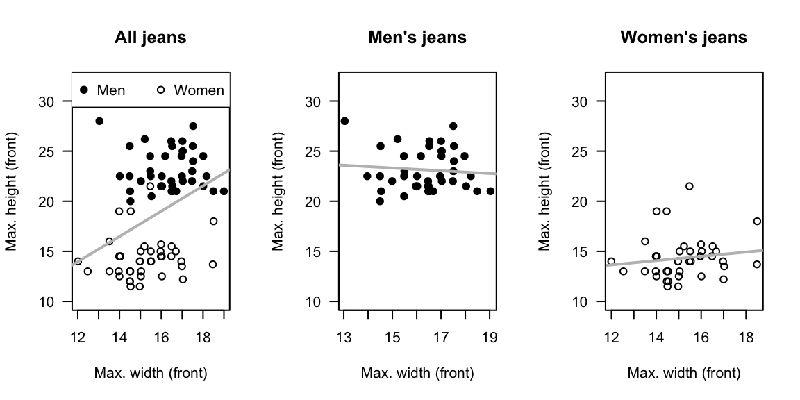
FIGURE 37.11: The relationships between minimum and maximum heights of front pockets for all jeans (left), men's jeans (centre) and women's jeans (right).

Exercise 37.12 [Dataset: Typing] The Typing dataset contains four variables: typing speed (mTS), typing accuracy (mAcc), age (Age). and sex (Sex) for \(1301\) students (Pinet et al. 2022). Is there evidence of a linear relationship between the mean typing speed and mean accuracy? Explain.

---

Peter K. Dunn, 2024: CC BY-NC-SA 4.0