27 CIs for comparing two independent means

So far, you have learnt to ask a RQ, design a study, classify and summarise the data, and form confidence intervals. In this chapter, you will learn to:

• identify situations where estimating a difference between two means is appropriate.
• construct confidence intervals for the difference between two independent means.
• determine whether the conditions for using the confidence intervals apply in a given situation.

27.1 Introduction: reaction times

Strayer and Johnston (2001) examined the reaction times, while driving, for students from the University of Utah (Agresti and Franklin 2007). In one study, students were randomly allocated to one of two groups: one group used a mobile phone while driving in a driving simulator, and one group did not use a mobile phone while driving in a driving simulator. The reaction time for each student was measured. This is a between-individuals comparison, since different students are in each group. (The study would be paired if each student's reaction time was measured twice: once using a phone, and once without using a phone.)

Consider this RQ:

For students, what is the difference between the mean reaction time while driving when using a mobile phone and when not using a mobile phone?

The data are shown below.

27.2 Notation

Since two groups are being compared, the two groups are distinguished using subscripts (Table 27.1). For the reaction-time data, we use the subscript \(P\) for the phone-users group, and \(C\) for the control (non-phone users) group.

Using this notation, the difference between population means (the parameter) is \((\mu_P - \mu_C)\). Since the population means are unknown, this parameter is estimated using the statistic \((\bar{x}_P - \bar{x}_C)\). The differences could be computed in the opposite direction (\(\bar{x}_C - \bar{x}_P\)). However, computing differences as the reaction time for phone users, minus the reaction time for non-phone users (controls) probably makes more sense: the differences then refer to the increase in the mean reaction times when students are using phones.

Be clear about how differences are defined! The differences could be computed as:

• the reaction time for phone users, minus the reaction time for non-phone users; this measures how much faster the reaction times is for non-phone users; or
• the reaction time for non-phone users, minus the reaction time for phone users; this measures how much faster the reaction times is for phone users.

Either is fine, provided you are consistent, and clear about how the difference are computed. The meaning of any conclusions will be the same.

TABLE 27.1: Notation used to distinguish between the two independent groups using subscripts. Any two subscripts can be used.

	group \(P\)	group \(C\)	(\(P - C\))
Population means:	\(\mu_P\)	\(\mu_C\)	\(\mu_P - \mu_C\)
Sample means:	\(\bar{x}_P\)	\(\bar{x}_C\)	\(\bar{x}_P - \bar{x}_C\)
Standard deviations:	\(s_P\)	\(s_C\)
Sample sizes:	\(n_P\)	\(n_C\)
Standard errors:	\(\displaystyle\text{s.e.}(\bar{x}_P) = \frac{s_P}{\sqrt{n_P}}\)	\(\displaystyle\text{s.e.}(\bar{x}_C) = \frac{s_C}{\sqrt{n_C}}\)	\(\displaystyle\text{s.e.}(\bar{x}_P - \bar{x}_C)\)

Table 27.1 does not include a standard deviation or a sample size for the difference between means. These make no sense in this context: no set of data exists for which a standard deviation or sample size can be found. For example, Group \(P\) has \(32\) individuals, and Group \(C\) has \(32\) individuals, but the sample size for the difference is not \(32 - 32 = 0\); there are just two samples of given sizes. However, the standard error of the difference between the means does make sense, as the value of \(\bar{x}_P - \bar{x}_C\) varies across all possible samples and so has a sampling distribution.

27.3 Summarising data

A suitable graphical summary of the data is a boxplot (Fig. 27.1, left panel), which shows that the sample medians are slightly different, and the IQRs slightly smaller, for the phone-using group. One large outlier is present for the phone-using group.

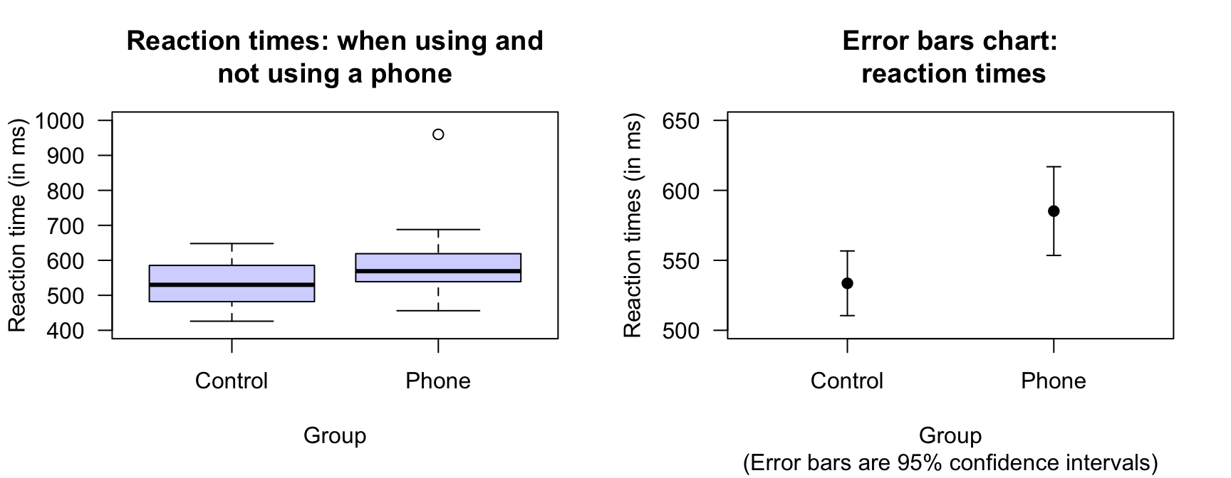
FIGURE 27.1: Left: boxplot of the two groups in the reaction-time data. Right: error bar chart comparing the mean reaction time for students not using a mobile phone (control), and using a mobile phone. The vertical scale is different for the two graphs.

The numerical summary of the data should summarise both groups (i.e., the first two rows of Table 27.2) The differences between the means is crucial (i.e., the third row), since the RQ is about this difference. The information can be found, for example, using software (Fig. 27.2).

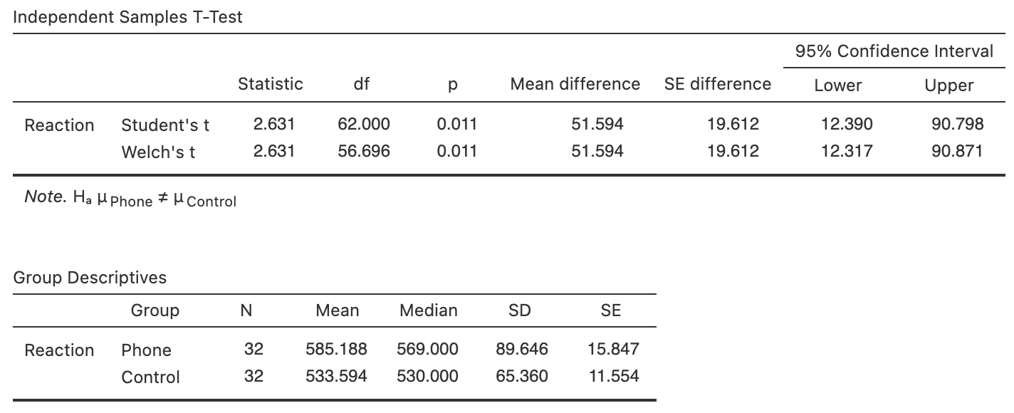
FIGURE 27.2: Software output for the phone reaction time data. The top table includes summaries of the difference between the two means, and the bottom table shows summaries for each group separately.

TABLE 27.2: Summary statistics for the reaction-time data (reaction times measured in ms).

	Mean	Sample size	Standard dev	Standard error
Not using phone	\(533.59\)	\(32\)	\(65.36\)	\(11.554\)
Using phone	\(585.19\)	\(32\)	\(89.65\)	\(15.847\)
Difference	\(\phantom{0}51.59\)			\(19.612\)

27.4 Error bar charts

A useful way to compare the means of two (or more) groups is to display the CIs for the means of the groups being compared in an error bar chart. Error bars charts display the expected variation in the sample means from sample to sample, while boxplots display the variation in the individual observations. For the reaction time data, the error bar chart (Fig. 27.1, right panel) shows the \(95\)% CI for each group; the mean has been added as a dot.

Example 27.1 (Error bar charts) Schepaschenko et al. (2017a) studied the foliage biomass of small-leaved lime trees from three sources: coppices; natural; planted. Three graphical summaries are shown in Fig. 27.3: a boxplot (showing the variation in individual trees; left), an error bar chart (showing the variation in the sample means; centre) on the same vertical scale as the boxplot, and the same error bar chart using a more appropriate scale for the error bar plot (right).

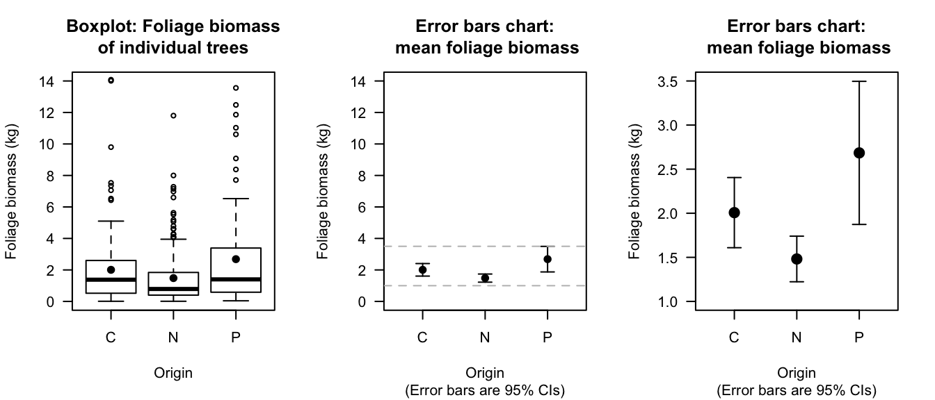
FIGURE 27.3: Boxplot (left) and error bar charts (centre; right) comparing the mean foliage biomass for small-leaved lime trees from three sources (C: Coppice; N: Natural; P: Planted). The centre panel shows an error bar chart using the same vertical scale as the boxplot; the dashed horizontal lines are the limits of the error bar chart on the right. The right error bar chart uses a more appropriate scale on the vertical axis. The solid dots show the mean of the distributions.

27.5 Confidence intervals for \(\mu_1 - \mu_2\)

Each sample will comprise different students, and give different reaction times. The sample means for each group will differ from sample to sample, and the difference between the sample means will be different for each sample. The difference between the sample means varies from sample to sample, and so has a sampling distribution and standard error.

Definition 27.1 (Sampling distribution for the difference between two sample means) The sampling distribution of the difference between two sample means \(\bar{x}_A\) and \(\bar{x}_B\) is (when the appropriate conditions are met; Sect. 27.6) described by:

• an approximate normal distribution,
• centred around a sampling mean whose value is \({\mu_{A}} - {\mu_{B}}\), the difference between the population means,
• with a standard deviation, called the standard error of the difference between the means, of \(\displaystyle\text{s.e.}(\bar{x}_A - \bar{x}_B)\).

The standard error for the difference between the means is found using \[ \text{s.e.}(\bar{x}_A - \bar{x}_B) = \sqrt{ \text{s.e.}(\bar{x}_A)^2 + \text{s.e.}(\bar{x}_B)^2}, \] though this value will often be given (e.g., on computer output).

For the reaction-time data, the differences between the sample means will have:

• an approximate normal distribution,
• centred around the sampling mean whose value is \(\mu_P - \mu_C\),
• with a standard deviation, called the standard error of the difference, of \(\text{s.e.}(\bar{x}_P - \bar{x}_C) = 19.612\).

The standard error of the difference between the means was computed using \[ \text{s.e.}(\bar{x}_A - \bar{x}_B) = \sqrt{ \text{s.e.}(\bar{x}_A)^2 + \text{s.e.}(\bar{x}_B)^2} = \sqrt{ 11.554^2 + 15.847^2 } = 19.612, \] as in the software output (Fig. 27.2).

The sampling distribution describes how the values of \(\bar{x}_P - \bar{x}_C\) vary from sample to sample. Then, finding a \(95\)% CI for the difference between the mean reaction times is similar to the process used in Chap. 24, since the sampling distribution has an approximate normal distribution: \[ \text{statistic} \pm \big(\text{multiplier} \times\text{s.e.}(\text{statistic})\big). \] When the statistic is \(\bar{x}_P - \bar{x}_C\), the approximate \(95\)% CI is \[ (\bar{x}_P - \bar{x}_C) \pm \big(2 \times \text{s.e.}(\bar{x}_P - \bar{x}_C)\big). \] So, in this case, the approximate \(95\)% CI is \[ 51.594 \pm (2 \times 19.612), \] or \(51.59\pm 19.61\), after rounding appropriately. We write:

The difference between reactions times is \(51.59\), slower for those using a phone (mean: \(585.19\); s.e.: \(15.85\); \(n = 32\)) compared to those not using a phone (mean: \(533.59\); s.e.: \(11.55\); \(n = 32\)), with an approximate \(95\)% CI for the difference between mean reaction times from \(12.37\) to \(90.82\).

The plausible values for the difference between the two population means are between \(12.37\) to \(90.82\)(slower for those using a phone).

Giving the CI alone is insufficient; the direction in which the differences were calculated must be given, so readers know which group had the higher mean.

Output from software often shows two CIs (Fig. 27.2). We will use the results from Welch's test (the second row), as this row of output is more general, and makes fewer assumptions. Specifically, the information in the first row (Student's t) is appropriate when the population standard deviations in the two groups are the same; the second row (Welch's t) is appropriate when the population standard deviations in the two groups are not necessarily the same. The information in the second row assumes less, and is more widely applicable.

Most software gives two confidence intervals: one assuming the standard deviations in the two groups are the same, and another not assuming the standard deviations in the two groups are the same.

We will use the information that does not assume the standard deviations in the two groups are the same. In the software output in Fig. 27.2, this is the second row of the top table (labelled 'Welch's \(t\)'). (The information in both rows are often similar anyway.)

From the output, the \(95\)% CI is from \(12.32\) to \(90.87\). The approximate CI and the exact (from software) CIs are only slightly different, as the samples sizes are not too small. (Recall: the \(t\)-multiplier of \(2\) is an approximation, based on the \(68\)--\(95\)--\(99.7\) rule).

27.6 Statistical validity conditions

As usual, these results apply under certain conditions. Statistical validity can be assessed using these criteria:

• When both samples have \(n \ge 25\), the CI is statistically valid. (If the distribution of a sample is highly skewed, the sample size for that sample may need to be larger.)
• When one or both groups have \(25\) or fewer observations, the CI is statistically valid only if the populations corresponding to both comparison groups have an approximate normal distribution.

The sample size of \(25\) is a rough figure; some books give other values (such as \(30\)). The histograms of the samples could be used to determine if normality of the populations seems reasonable. The units of analysis are also assumed to be independent (e.g., from a simple random sample).

If the statistical validity conditions are not met, other methods (e.g., non-parametric methods (Conover 2003); resampling methods (Efron and Hastie 2021)) may be used.

Example 27.2 (Statistical validity) For the reaction-time data, both samples are larger than \(25\), so the CI is statistically valid. Note that the phone-users group has a large outlier, so the sample size being larger than \(25\) is probably necessary.

27.7 Example: speed signage

To reduce vehicle speeds on freeway exit ramps, Ma et al. (2019) studied adding additional signage. At one site (Ningxuan Freeway), speeds were recorded for \(38\) vehicles before the extra signage was added, and then for \(41\) different vehicles after the extra signage was added.

The researchers are hoping that the addition of extra signage will reduce the mean speed of the vehicles. The RQ is:

At this freeway exit, how much is the mean vehicle speed reduced after extra signage is added?

The data are not paired: different vehicles are measured before (\(B\)) and after (\(A\)) the extra signage is added. The data can be summarised (Table 27.3) using the software output (Fig. 27.4). Define \(\mu\) as the mean speed (in km.h^\(-1\)) on the exit ramp, and the parameter as \(\mu_B - \mu_A\), the reduction in the mean speed.

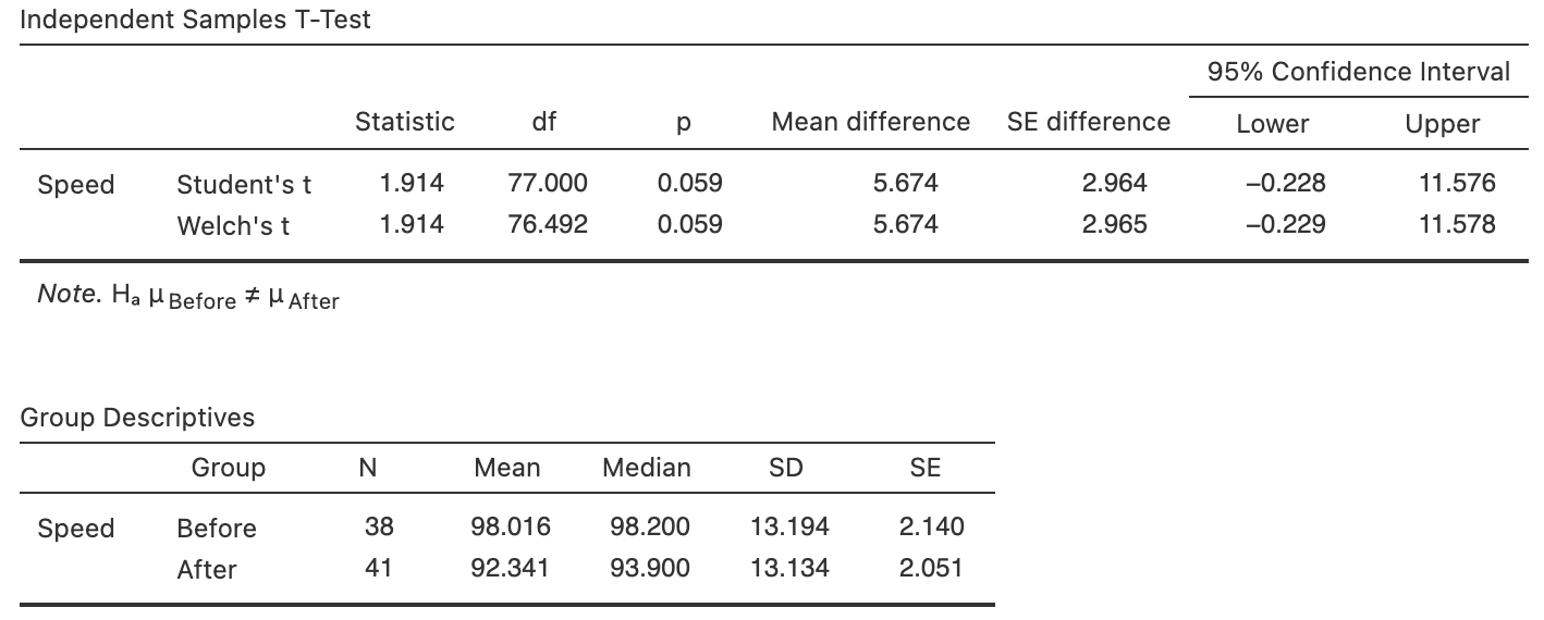
FIGURE 27.4: Software output for the speed data.

TABLE 27.3: The signage data summary (in km.h\(^{-1}\)).

	Mean	Median	Standard deviation	Standard error	Sample size
Before	\(98.02\)	\(98.2\)	\(13.19\)	\(\phantom{0}2.1\)	\(38\)
After	\(92.34\)	\(93.9\)	\(13.13\)	\(\phantom{0}2.1\)	\(41\)
Speed reduction	\(\phantom{0}5.68\)

The standard error of the difference is \[ \text{s.e.}(\bar{x}_A - \bar{x}_B) = \sqrt{ \text{s.e.}(\bar{x}_A)^2 + \text{s.e.}(\bar{x}_B)^2 } = \sqrt{ 2.05124^2 + 2.14031^2 } = 2.96454, \] as in the second row ('Welch's \(t\)') of the first table in Fig. 27.4.

A useful graphical summary of the data is a boxplot (Fig. 27.5, left panel); likewise, an error bar chart can be produced to compare the means (Fig. 27.5, right panel).

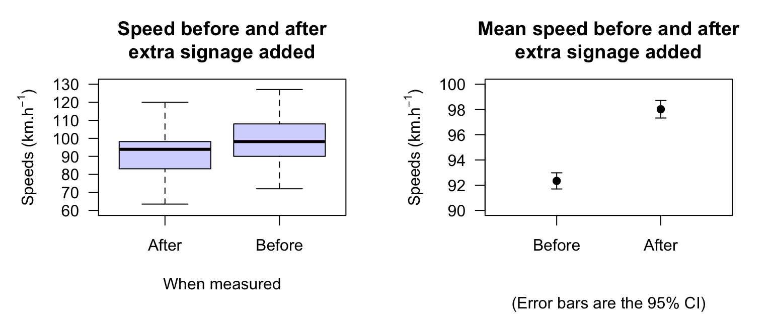
FIGURE 27.5: Boxplot (left) and error bar chart (right) showing the mean speed before and after the addition of extra signage, and the \(95\)% CIs. The vertical scales on the two graphs are different.

Based on the sample, an approximate \(95\)% CI for the difference in mean speeds is \(5.68 \pm (2 \times 2.964)\), or from \(-0.24\) to \(11.6\).h^\(-1\), higher before the addition of extra signage. (The negative value refers to a negative reduction; that is, an increase in speed of \(0.24\).h^\(-1\).)

From Fig. 27.4, a \(95\)% CI is from \(-11.6\) to \(0.23\).h^\(-1\), lower before the addition of extra signage (since the After information is given first in the second table of Fig. 27.4). This is equivalent to a \(95\)% CI from \(-0.23\) to \(11.6\).h^\(-1\), higher before the addition of extra signage. The exact and approximate \(95\)% CIs are almost exactly the same.

The CI means that, if many samples of size \(38\) and \(41\) were found, and the difference between the mean speeds were found, about \(95\)% of the CIs would contain the population difference (\(\mu_A - \mu_A\)). Loosely speaking, there is a \(95\)% chance that our CI straddles the difference in the population means (\(\mu_B - \mu_A\)).

We could write:

The reduction in the mean speed after adding signage is \(5.68\).h^\(-1\) (before mean: \(98.02\); s.e.: \(2.140\); \(n = 38\); after mean: \(92.34\); s.e.: \(2.051\); \(n = 41\)), with a \(95\)% CI between \(-0.24\) km.h^\(-1\) (i.e., an increase of \(0.23\).h^\(-1\)) and \(11.6\).h^\(-1\) (two independent samples).

Using the validity conditions, the CI is statistically valid.

Remember: clearly state which mean is larger.

27.8 Example: chamomile tea

(This study was seen in Sect. 26.7.) Rafraf, Zemestani, and Asghari-Jafarabadi (2015) studied patients with Type 2 diabetes mellitus (T2DM). They randomly allocated \(32\) patients into a control group (who drank hot water), and \(32\) to receive chamomile tea.

The total glucose (TG) was measured for each individual, in both groups, before the intervention and after eight weeks on the intervention. The data are not available, so a graphical summary of the data cannot be produced. However, a data summary is given in the article (motivating Table 26.3).

The following relational RQ can be asked:

For patients with T2DM, what is the mean difference between the average reductions in TG, comparing those drinking chamomile tea and those who drink hot water?

Here, two separate groups are being compared: the tea-drinking group (\(T\)), and the control water-drinking group (\(W\)). Defining \(\mu\) as the mean reduction in TG, the differences between the TG reductions in the two groups is \(\mu_T - \mu_W\). (Of course, the difference can be defined either way, provided we are consistent.) In Sect. 26.7, the mean reduction in each group was estimated. From Table 26.3, the estimate of the mean difference is \(\bar{x}_T - \bar{x}_W = 45.74\).dl^\(-1\). The standard error can be determined from the information in the first two rows of the data summary table: \(\text{s.e.}(\bar{x}_T - \bar{x}_W) = 8.42\). Hence, an approximate \(95\)% CI for the difference between the mean reduction is \[ 45.74 \pm (2\times 8.42), \] or from \(28.90\) to \(62.58\).dl^\(-1\), with a larger reduction for the tea group. This is a CI for the difference between the mean reductions in each group. The approximate \(95\)% CIs for each group can also be computed, and an error bar chart produced (Fig. 27.6).

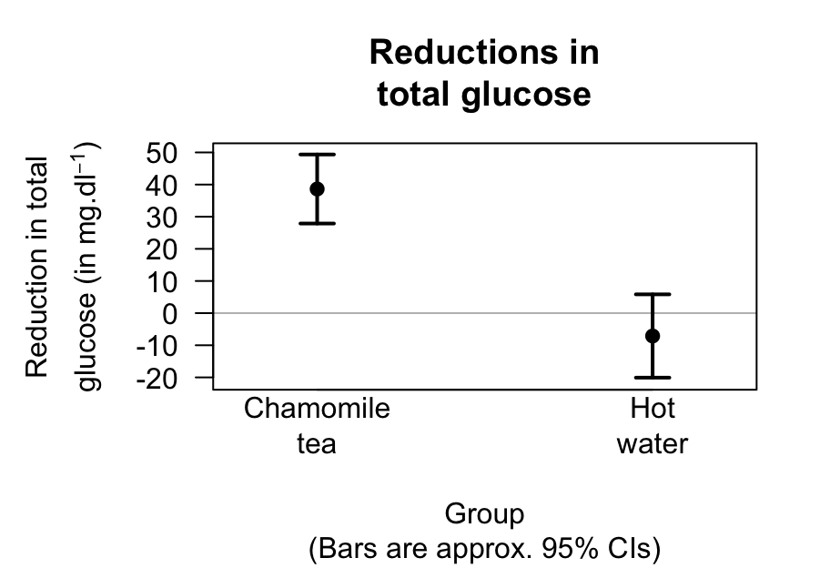
FIGURE 27.6: The reduction in total glucose for the chamomile-tea drinking group, and the control group. The horizontal grey line represented no mean reduction in TG in each group.

We write:

The difference between the mean reductions in TG is \(45.74\).dl^\(-1\), greater for the tea-drinking group, with the approximate \(95\)% CI from \(28.64\) to \(62.84\).dl^\(-1\).

This interval has a \(95\)% chance of straddling the difference between the mean reductions in TG. The sample sizes are larger than \(25\) (\(n = 32\) for both groups), so the results are statistically valid.

27.9 Chapter summary

To compute a confidence interval (CI) for the difference between two means, compute the difference between the two sample mean, \(\bar{x}_A - \bar{x}_B\), and identify the sample sizes \(n_A\) and \(n_B\). Then compute the standard error, which quantifies how much the value of \(\bar{x}_A - \bar{x}_B\) varies across all possible samples: \[ \text{s.e.}(\bar{x}_A - \bar{x}_B) = \sqrt{ \text{s.e}(\bar{x}_A) + \text{s.e.}(\bar{x}_B)}, \] where \(\text{s.e.}(\bar{x}_A)\) and \(\text{s.e.}(\bar{x}_B)\) are the standard errors of Groups \(A\) and \(B\). The margin of error is (multiplier\({}\times{}\)standard error), where the multiplier is \(2\) for an approximate \(95\)% CI (using the \(68\)--\(95\)--\(99.7\) rule). Then the CI is: \[ (\bar{x}_A - \bar{x}_B) \pm \left( \text{multiplier}\times\text{standard error} \right). \] The statistical validity conditions should also be checked.

27.10 Quick review questions

1. What is an appropriate graph for displaying quantitative data for two separate groups?
   boxplothistogramside-by-side bar charterror bar chart
2. True or false: The difference in population means could be denoted by \(\mu_A - \mu_B\).
   TRUE FALSE
3. True or false: The standard error of the difference between the sample means is denoted by \(\text{s.e.}(\bar{x}_A) - \text{s.e.}(\bar{x}_B)\).
   TRUE FALSE
4. True or false: An error bar chart displays the variation in the data.
   TRUE FALSE

27.11 Exercises

Answers to odd-numbered exercises are available in App. E.

Exercise 27.1 Agbayani, Fortune, and Trites (2020) measured (among other things) the length of gray whales (Eschrichtius robustus) at birth. How much longer are male gray whales than females, on average, in the population? Summary data are given in Table 27.4.

TABLE 27.4: Numerical summary of length of whales at birth (in m).

	Mean	Standard deviation	Sample size
Female	\(4.60\)	\(0.305\)	\(30\)
Male	\(4.66\)	\(0.379\)	\(26\)

1. Define the parameter, and write down its estimate.
2. Sketch an error bar chart.
3. Compute the standard error of the difference between the two means.
4. Compile a numerical summary table.
5. Compute the approximate \(95\)% CI, and write a conclusion.
6. Is the CI statistically valid?

Exercise 27.2 [Dataset: NHANES] The NHANES study records data annually about a representative sample of Americans. The data can be used to answer the RQ:

Among Americans, is the mean direct HDL cholesterol different for current smokers and non-smokers?

Use the software output (Fig. 27.7) to answer these questions.

1. Define the parameter of interest, and write down its estimate.
2. Sketch an error bar chart.
3. Compile a numerical summary table.
4. Compute the approximate \(95\)% CI, and write a conclusion.
5. Write down the exact \(95\)% CI, and write a conclusion.
6. Is the CI statistically valid?

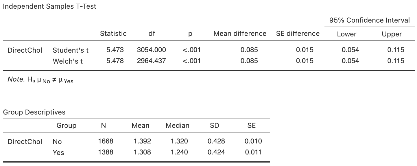
FIGURE 27.7: Software output for the NHANES data.

Exercise 27.3 Barrett et al. (2010) studied the effectiveness of echinacea to treat the common cold. They compared, among other things, the duration of the cold for participants treated with echinacea or a placebo. Participants were blinded to the treatment, and allocated to the groups randomly. A summary of the data is given in Table 27.5.

1. Compute the standard error for the mean duration of symptoms for each group.
2. Compute the standard error for the difference between the means.
3. Sketch an error bar chart.
4. Compute an approximate \(95\)% CI for the difference between the mean durations for the two groups.
5. In which direction is the difference computed? What does it mean when the difference is calculated in this way?
6. Compute an approximate \(95\)% CI for the population mean duration of symptoms for those treated with echinacea.
7. Are the CIs statistically valid?
8. Is the difference likely to be of practical importance?

TABLE 27.5: Numerical summary of duration (in days) of common cold symptoms, for blinded patients taking echinacea or a placebo.

	Mean	Standard deviation	Standard error	Sample size
Placebo	\(6.87\)	\(3.62\)		\(176\)
Echinacea	\(6.34\)	\(3.31\)		\(183\)
Difference	\(0.53\)

Exercise 27.4 Carpal tunnel syndrome (CTS) is pain experienced in the wrists. Schmid et al. (2012) compared two different treatments: night splinting, or gliding exercises.

Participants were randomly allocated to one of the two groups. Pain intensity (measured using a quantitative visual analog scale; larger values mean greater pain) were recorded after one week of treatment. The data are summarised in Table 27.6.

1. Compute the standard error for the mean pain intensity for each group.
2. Compute the standard error for the difference between the mean of the two groups.
3. In which direction is the difference computed? What does it mean when the difference is calculated in this way?
4. Compute an approximate \(95\)% CI for the difference in the mean pain intensity for the treatments.
5. Compute an approximate \(95\)% CI for the population mean pain intensity for those treated with splinting.
6. Are the CIs statistically valid?

TABLE 27.6: Numerical summary of pain intensity for two different treatments of carpal tunnel syndrome.

	Mean	Standard deviation	Standard error	Sample size
Exercise	\(0.8\)	\(1.4\)		\(10\)
Splinting	\(1.1\)	\(1.1\)		\(10\)
Difference	\(0.3\)

Exercise 27.5 Sketch the sampling distribution for the difference between the mean reaction times for students using their phone while driving, and students not using their phone while driving.

Exercise 27.6 Sketch the sampling distribution for the difference between the mean speeds before and after adding extra signage, in Sect. 27.7.

Exercise 27.7 [Dataset: Dental] Woodward and Walker (1994) recorded the sugar consumption in industrialised countries (mean: \(41.8\)/person/year) and non-industrialised countries (mean: \(24.6\)/person/year). Using the software output (Fig. 27.8), write down and interpret the CI.

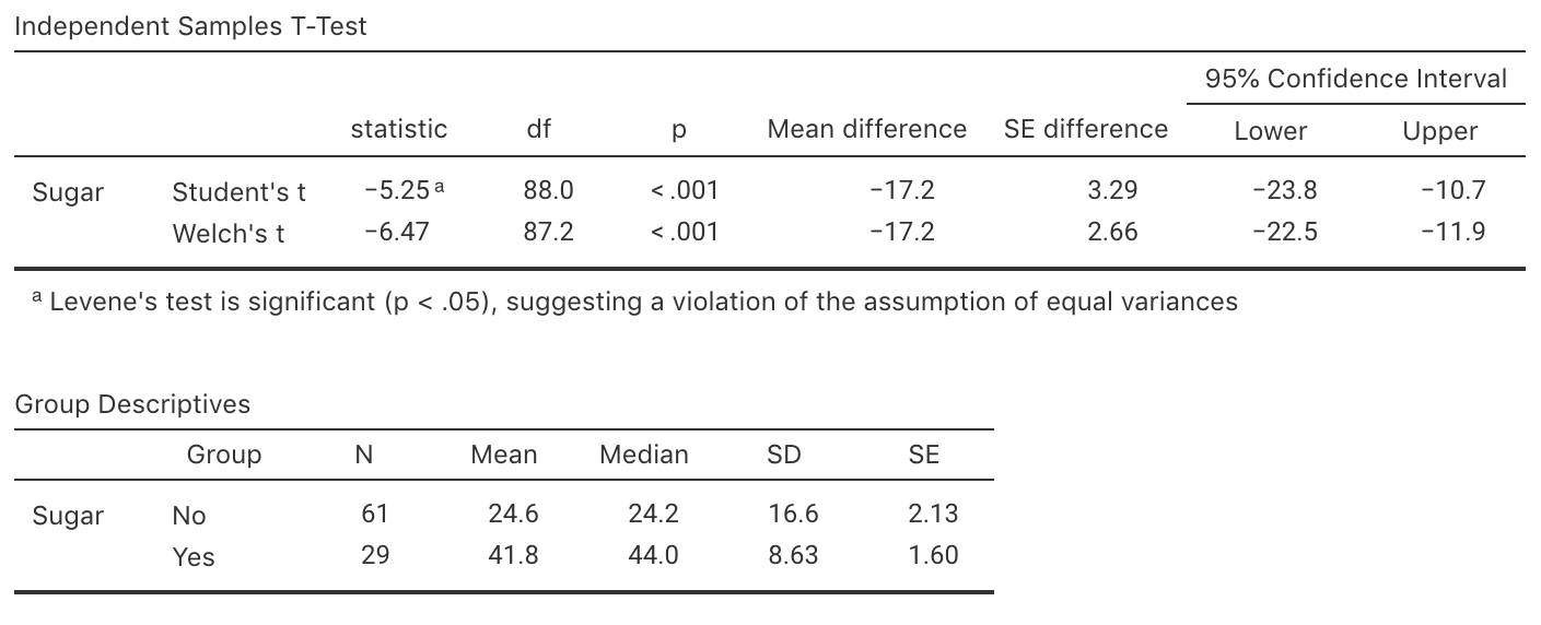
FIGURE 27.8: Software output for the sugar-consumption data; the Groups refer to whether or not the country is industrialised.

Exercise 27.8 [Dataset: Deceleration] To reduce vehicle speeds on freeway exit ramps, Ma et al. (2019) studied using additional signage. At one site (Ningxuan Freeway), the deceleration of vehicles was recorded at various points on the freeway exit for \(38\) vehicles before the extra signage was added, and then for \(41\) vehicles after the extra signage was added (Exercise 15.10) as the vehicle left the \(120\).h^\(-1\) speed zone and approached the \(80\).h^\(-1\) speed zone. Use the data, and the summary in Exercise 15.10 to address this RQ:

At this freeway exit, what is the difference between the mean vehicle deceleration, comparing the times before the extra signage is added and after extra signage is added?

In this context, the researchers are hoping that the extra signage might cause cars to slow down faster (i.e., greater deceleration, on average, after adding the extra signage).

1. Identify clearly the parameter of interest to understand how much the deceleration increased after adding the extra signage.
2. Compute and interpret the CI for this parameter.

Exercise 27.9 [Dataset: ForwardFall] Wojcik et al. (1999) compared the lean-forward angle in younger and older women. An elaborate set-up was constructed to measure this angle, using a harnesses. Consider the RQ:

Among healthy women, what is difference between the mean lean-forward angle for younger women compared to older women?

The data are shown in Table 15.6.

1. What is the parameter? Describe what this means.
2. What is an appropriate graph to display the data?
3. Construct an appropriate numerical summary from the software output (Fig. 27.9).
4. Construct approximate and exact \(95\)% CIs. Explain any differences.
5. Is the CI expected to be statistically valid?
6. Write a conclusion.

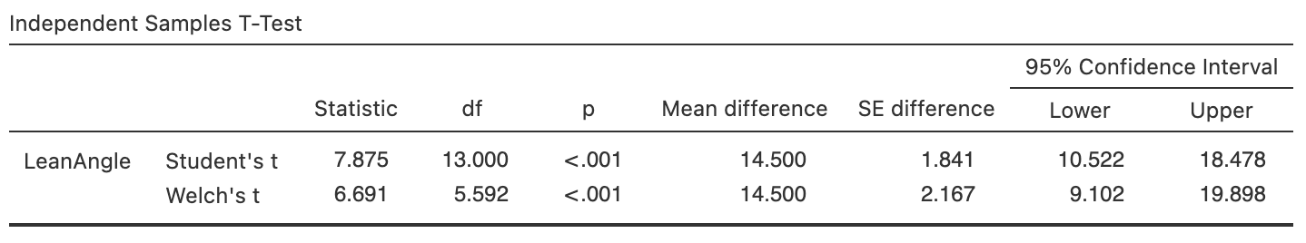
FIGURE 27.9: Software output for the lean-forward angles data.

Exercise 27.10 Becker, Stuifbergen, and Sands (1991) compared the access to health promotion (HP) services for people with and without a disability in southwestern of the USA. 'Access' was measured using the quantitative Barriers to Health Promoting Activities for Disabled Persons (BHADP) scale. Higher scores mean greater barriers to health promotion services. The RQ is:

What is the difference between the mean BHADP scores, for people with and without a disability, in southwestern USA?

1. Define the parameter, and write down its estimate.
2. Sketch an error bar chart.
3. Compute the standard error of the difference.
4. Compile a numerical summary table.
5. Compute the approximate \(95\)% CI, and write a conclusion.
6. Is the CI statistically valid?

TABLE 27.7: The data summary for BHADP scores (no measurement units).

	Sample mean	Standard deviation	Sample size	Standard error
Disability	\(31.83\)	\(7.73\)	\(132\)	\(0.67280\)
No disability	\(25.07\)	\(4.80\)	\(137\)	\(0.41010\)
Difference	\(\phantom{0}6.76\)

Exercise 27.11 [Dataset: BodyTemp] The average internal body temperature is commonly believed to be \(37.0^\circ\text{C}\) (\(98.6\)^oF). Mackowiak, Wasserman, and Levine (1992) wished to determine the difference between the mean internal body temperature for males and females. Use the software output in Fig. 27.10 to construct an approximate \(95\)% CI appropriate for answering the RQ.

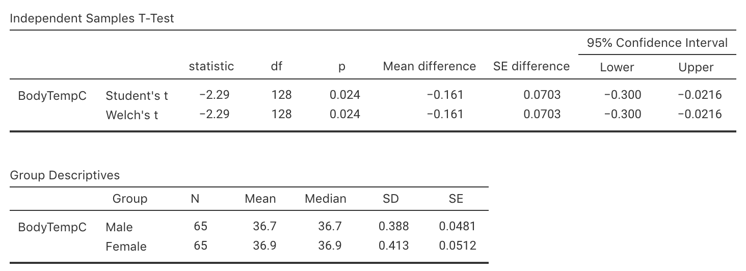
FIGURE 27.10: Software output for the body-temperature data.

Exercise 27.12 D. Chapman et al. (2007) compared 'conventional' male paramedics in Western Australia with male special-operations paramedics. Some information comparing their physical profiles is shown in Table 27.8.

1. Compute the missing standard errors.
2. Compute an approximate \(95\)% CI for the difference in the mean grip strength for the two groups of paramedics.
3. Compute an approximate \(95\)% CI for the difference between the number of push-ups for the two groups of paramedics.
4. Discuss the conditions required for statistical validity.

TABLE 27.8: The physical profile of conventional (\(n = 18\)) and special operation (\(n = 11\)) paramedics in Western Australia.

	Conventional	Special Operations
Grip strength (in kg)
Mean	\(51\)	\(56\)
Standard deviation	\(\phantom{0}8\)	\(\phantom{0}9\)
Standard error
Push-ups (per minutes)
Mean	\(36\)	\(47\)
Standard deviation	\(10\)	\(11\)
Standard error

Exercise 27.13 [Dataset: Anorexia] Young girls (\(n = 29\)) with anorexia received cognitive behavioural treatment (Hand et al. (1996)), while another \(n = 26\) young girls received a control treatment (the 'standard' treatment). All girls had their weight recorded before and after treatment.

1. Determine the mean gain in each individuals girls weight using software.
2. Compute a CI for the mean weight gain for the girls in each group.
3. Compute a CI for the mean difference between the weight gains for the two treatment groups.

Exercise 27.14 Researchers studied the impact of a gluten-free diet on dental cavities (Khalaf et al. 2020). Some of the summary information regarding the number decayed, missing and filled teeth (DMFT) is shown in Table 27.9. An exact \(95\)% CI is given as for the difference is \(-2.32\) to \(2.76\).

1. Using the \(68\)--\(95\)--\(99.7\) rule gives a slightly different CI. Why?

2. True or false: the difference is computed as the number of DMFT for coeliacs minus non-coeliacs.

3. True or false: one of the values for the CI is a negative value, which must be an error (as a negative number of DMFT is impossible).

4. We are \(95\)% confidence that the difference between the population means is:

   • Smaller for coeliacs;
   • Between 2.32 higher for non-coeliacs to 2.76 higher for coeliacs.
   • Between 2.76 higher for non-coeliacs to 2.32 higher for coeliacs.

TABLE 27.9: The summary of the number of DMFT for coeliacs and non-coeliacs.

	Sample size	Mean	Standard deviation	Standard error
Coeliacs	\(23\)	\(8.39\)	\(4.4\)	\(0.92\)
Non-coeliacs	\(23\)	\(8.17\)	\(4.1\)	\(0.86\)
Difference		\(0.22\)		\(1.30\)

---

Peter K. Dunn, 2024: CC BY-NC-SA 4.0