Chapter 9 Considering Prior Distributions

One of the most commonly asked questions when one first encounters Bayesian statistics is “how do we choose a prior?” While there is never one “perfect” prior in any situation, we’ll discuss in this chapter some issues to consider when choosing a prior. But first, here are a few big picture ideas to keep in mind.

Bayesian inference is based on the posterior distribution, not the prior. Therefore, the posterior requires much more attention than the prior.
The prior is only one part of the Bayesian model. The likelihood is the other part. And there is the data that is used to fit the model. Choice of prior is just one of many modeling assumptions that should be evaluated and checked.
In many situations, the posterior distribution is not too sensitive to reasonable changes in prior. In these situations, the important question isn’t “what is the prior?” but rather “is there a prior at all”? That is, are you adopting a Bayesian approach, treating parameters as random variables, and quantifying uncertainty about parameters with probability distributions?
One criticism of Bayesian statistics in general and priors in particular is that they are subjective. However, any statistical analysis is inherently subjective, filled with many assumptions and decisions along the way. Except in the simplest situations, if you ask five statisticians how to approach a particular problem, you will likely get five different answers. Priors and Bayesian data analysis are no more inherently subjective than any of the myriad other assumptions made in statistical analysis.

Subjectivity is OK, and often beneficial. Choosing a subjective prior allows us to explicitly incorporate a wealth of past experience into our analysis.

Example 9.1 Xiomara claims that she can predict which way a coin flip will land. Rogelio claims that he can taste the difference between Coke and Pepsi.

Before reading further, stop to consider: whose claim - Xiomara’s or Rogelio’s - is initially more convincing? Or are you equally convinced? Why? To put it another way, whose claim are you initially more skeptical of? Or are you equally skeptical? To put it one more way, whose claim would require more data to convince you?¹⁷

To test Xiomara’s claim, you flip a fair coin 10 times, and she correctly predicts the result of 9 of the 10 flips. (You can assume the coin is fair, the flips are independent, and there is no funny business in data collection.)

To test Rogelio’s claim, you give him a blind taste test of 10 cups, flipping a coin for each cup to determine whether to serve Coke or Pespi. Rogelio correctly identifies 9 of the 10 cups. (You can assume the coin is fair, the flips are independent, and there is no funny business in data collection.)

Let \(\theta_X\) be the probability that Xiomara correctly guesses the result of a fair coin flip. Let \(\theta_R\) be the probability that Rogelio correctly guesses the soda (Coke or Pepsi) in a randomly selected cup.

How might a frequentist address this situation? What would the conclusion be?
Consider a Bayesian approach. Describe, in general terms, your prior distributions for the two parameters. How do they compare? How would this impact your conclusions?

\iffalse{} Solution. to Example 9.1

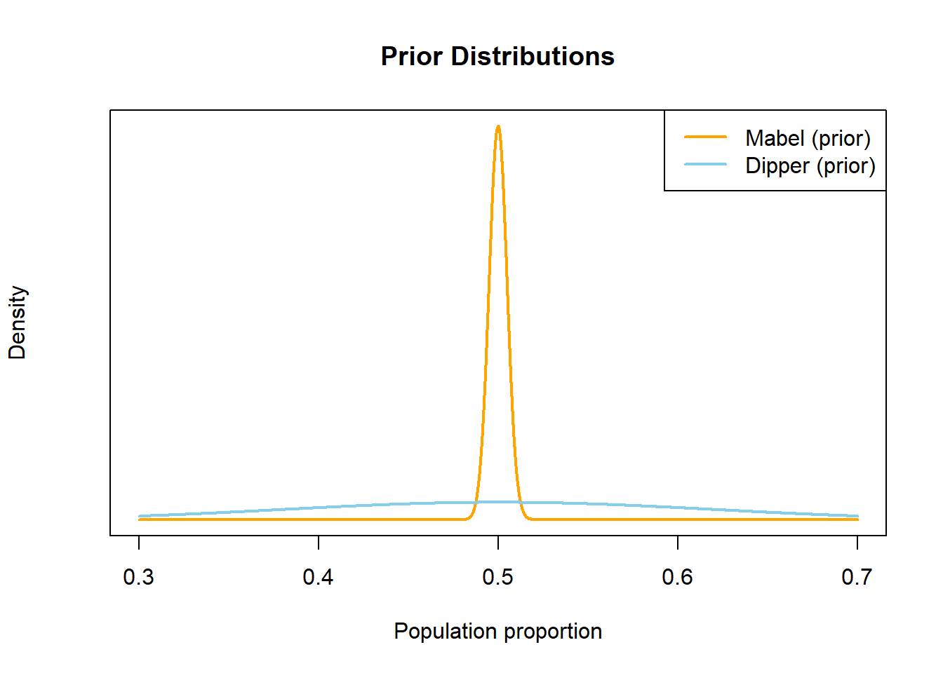
For Xiomara, a frequentist might conduct a hypothesis test of the null hypothesis \(H_0:\theta_X = 0.5\) versus the alternative hypothesis: \(H_a:\theta_X > 0.5\). The p-value would be about 0.01, the probability of observing at least 9 out of 10 successes from a Binomial distribution with parameters 10 and 0.5 (1 - pbinom(8, 10, 0.5)). Rogelio’s set up would be similar and would yield the same p-value. So a strict frequentist would be equally convinced of the two claims.
Prior to observing data, we are probably more skeptical of Xiomara’s claim than Rogelio’s. Since coin flips are unpredictable, we would have a strong prior belief that \(\theta_X\) is close to 0.5 (what it would be if she were just guessing). Our prior for \(\theta_X\) would have a mean of 0.5 and a small prior SD, to reflect that only values close to 0.5 seem plausible. Therefore, it would require a lot of evidence to sway our prior beliefs.
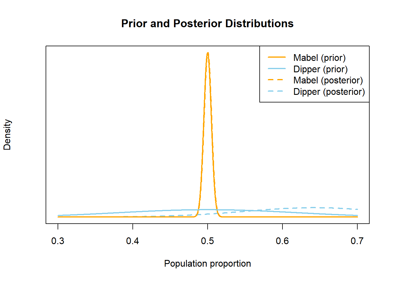
On the other hand, we might be familiar with people who can tell the difference between Coke and Pepsi; maybe we even can ourselves. Our prior for \(\theta_R\) would have a smaller prior SD than that of \(\theta_X\) to allow for a wider range of plausible values. We might even have a prior mean for \(\theta_R\) above 0.5 if we have experience with a lot of people who can tell the difference between Coke and Pepsi. Given the sample data, our posterior probability that \(\theta_R>0.5\) would be larger than the posterior probability that \(\theta_X > 0.5\), and we would be more convinced by Rogelio’s claim than by Xiomara’s.

Even if a prior does not represent strong prior beliefs, just having a prior distribution at all allows for Bayesian analysis. Remember, both Bayesian and frequentist are valid approaches to statistical analyses, each with advantages and disadvantages. That said, there are some issues with frequentist approaches that incorporating a prior distribution and adopting a Bayesian approach alleviates. (To be fair, an upcoming investigation will address some disadvantages of the Bayesian approach compared with the frequentist approach.)

Example 9.2 Tamika is a basketball player who throughout her career has had a probability of 0.5 of making any three point attempt. However, her coach is afraid that her three point shooting has gotten worse. To check this, the coach has Tamika shoot a series of three pointers; she makes 7 out of 24. Does the coach have evidence that Tamika has gotten worse?

Let \(\theta\) be the probability that Tamika successfully makes any three point attempt. Assume attempts are independent.

Prior to collecting data, the coach decides that he’ll have convincing evidence that Tamika has gotten worse if the p-value is less than 0.025. Suppose the coach told Tamika to shoot 24 attempts and then stop and count the number of successful attempts. Use software to compute the p-value. Is the coach convinced that Tamika has gotten worse?
Prior to collecting data, the coach decides that he’ll have convincing evidence that Tamika has gotten worse if the p-value is less than 0.025. Suppose the coach told Tamika to shoot until she makes 7 three pointers and then stop and count the number of total attempts. Use software to compute the p-value. Is the coach convinced that Tamika has gotten worse? (Hint: the total number of attempts has a Negative Binomial distribution.)
Now suppose the coach takes a Bayesian approach and assumes a Beta(\(\alpha\), \(\beta\)) prior distribution for \(\theta\). Suppose the coach told Tamika to shoot 24 attempts and then stop and count the number of successful attempts. Identify the likelihood function and the posterior distribution of \(\theta\).
Now suppose the coach takes a Bayesian approach and assumes a Beta(\(\alpha\), \(\beta\)) prior distribution for \(\theta\). Suppose the coach told Tamika to shoot until she makes 7 three pointers and then stop and count the number of total attempts. Identify the likelihood function and the posterior distribution of \(\theta\).
Compare the Bayesian and frequentist approaches in this example. Does the “strength of the evidence” depend on how the data were collected?

\iffalse{} Solution. to Example 9.2

The null hypothesis is \(H_0:\theta = 0.5\) and the alternative hypothesis is \(H_a:\theta < 0.5\). If the null hypothesis is true and Tamika has not gotten worse, then \(Y\), the number of successful attempts, has a Binomial(24, 0.5) distribution. The p-value is \(P(Y \le 7) = 0.032\) from pbinom(7, 24, 0.5). Using a strict threshold of 0.025, the coach has NOT been convinced that Tamika has gotten worse.
The null hypothesis is \(H_0:\theta = 0.5\) and the alternative hypothesis is \(H_a:\theta < 0.5\). If the null hypothesis is true and Tamika has not gotten worse, then \(N\), the number of total attempts required to achieve 7 successful attempts, has a Negative Binomial(7, 0.5) distribution. The p-value is \(P(N \ge 24) = 0.017\) from 1 - pnbinom(23 - 7, 7, 0.5). (In R, nbinom only counts the total number of failures, not the total number of trials.) Using a strict threshold of 0.025, the coach has been convinced that Tamika has gotten worse.
The data is \(Y\), the number of successful attempts in 24 attempts, which follows a Binomial(24, \(\theta\)) distribution. The likelihood is \(P(Y=7|\theta)\) \[ f(y=7|\theta) = \binom{24}{7}\theta^7(1-\theta)^{17} \propto \theta^{7}(1-\theta)^{17}, \qquad 0 < \theta < 1. \] The posterior distribution is the Beta(\(\alpha + 7\), \(\beta + 17\)) distribution.
The data is \(N\), the number of total attempts required to achieve 7 successful attempts, which follows a Negative Binomial(7, \(\theta\)) distribution. The likelihood is \(P(N=24|\theta)\) \[ f(n = 24|\theta) = \binom{24 - 1}{7 - 1}\theta^7(1-\theta)^{17} \propto \theta^{7}(1-\theta)^{17}, \qquad 0 < \theta < 1. \] (The \(\binom{24 - 1}{7 - 1}\) follows from the fact that the last attempt has to be success.) Note that the shape of the likelihood as a function of \(\theta\) is the same as in the previous part. Therefore, the posterior distribution is the Beta(\(\alpha + 7\), \(\beta + 17\)) distribution.
Even though both frequentist scenario involves 7 successes in 24 attempts, the p-value measuring the strength of the evidence to reject the null hypothesis differed depending on how the data were collected. Using a strict cutoff of 0.025 led the coach to reject the null hypothesis in one scenario but not the other. However, the Bayesian analysis is the same in either scenario since the posterior distributions were the same. For the Bayesian analysis, all that mattered about the data was that there were 7 successes in 24 attempts.

Bayesian data analysis treats parameters as random variables with probability distributions. The prior distribution quantifies the researcher’s uncertainty about parameters before observing data. Some issues to consider when choosing a prior include, in no particular order:

The researcher’s prior beliefs! A prior distribution is part of a statistical model, and should be consistent with knowledge about the underlying scientific problem. Researchers are often experts with a wealth of past experience that can be explicitly incorporated into the analysis via the prior distribution. Such a prior is called an informative or weakly informative prior.
A regularizing prior. A prior which, when tuned properly, reduces overfitting or “overreacting” to the data.
Noninformative prior a.k.a., (reference, vague, flat prior). A prior is sought that plays a minimal role in inference so that “the data can speak for itself”.
Mathematical convenience. The prior is chosen so that computation of the posterior is simplified, as in the case of conjugate priors.
Interpretation. The posterior is a compromise between the data and prior. Some priors allow for easy interpretation of the relative contributions of data and prior to the posterior. For example, think of the “prior successes and prior failures” interpretation in the Beta-Binomial model.
Prior based on past data. Bayesian updating can be viewed as an iterative process. The posterior distribution obtained from one round of data collection can inform the prior distribution for another round.

For those initially skeptical of prior distributions at all, the strategy of always choosing an noninformative or flat prior might be appealing. Flat priors are common, but are rarely ever the best choices from a modeling perspective. Just like you would not want to assume a Normal distribution for the likelihood in every problem, you would not to use a flat prior in every problem.

Furthermore, there are some subtle issues that arise when attempting to choose a noninformative prior.

Example 9.3 Suppose we want to estimate \(\theta\), the population proportion of Cal Poly students who wore socks at any point yesterday.

What are the possible values for \(\theta\)? What prior distribution might you consider a noninformative prior distribution?
You might choose a Uniform(0, 1) prior, a.k.a., a Beta(1, 1) prior. Recall how we interpreted the parameters \(\alpha\) and \(\beta\) in the Beta-Binomial model. Does the Beta(1, 1) distribution represent “no prior information”?
Suppose in a sample of 20 students, 4 wore socks yesterday. How would you estimate \(\theta\) with a single number based only on the data?
Assume a Beta(1, 1) prior and the 4/20 sample data. Identify the posterior distribution. Recall that one Bayesian point estimate of \(\theta\) is the posterior mean. Find the posterior mean of \(\theta\). Does this estimate let the “data speak entirely for itself”?
How could you change \(\alpha\) and \(\beta\) in the Beta distribution prior to represent no prior information? Sketch the prior. Do you see any potential problems?
Assume a Beta(0, 0) prior for \(\theta\) and the 4/20 sample data. Identify the posterior distribution. Find the posterior mode of \(\theta\). Does this estimate let the “data speak entirely for itself”?
Now suppose the parameter you want to estimate is the odds that a student wore socks yesterday, \(\phi=\frac{\theta}{1-\theta}\). What are the possible values of \(\phi\)? What might a non-informative prior look like? Is this a proper prior?
Assume a Beta(1, 1) prior for \(\theta\). Use simulation to approximate the prior distribution of the odds \(\phi\). Would you say this is a noninformative prior for \(\phi\)?

\iffalse{} Solution. to Example 9.3

\(\theta\) takes values in (0, 1). We might assume a flat prior on (0, 1), that is a Uniform(0, 1) prior.
We interpreted \(\alpha\) as “prior successes” and \(\beta\) as “prior failures”. So a Beta(1, 1) is in some some equivalent to a “prior sample size” of 2. Certainly not a lot of prior information, but it’s not “no prior information” either.
The sample proportion, 4/20 = 0.2.
With a Beta(1, 1) prior and the 4/20 sample data, the posterior distribution is Beta(5, 17). The posterior mean of \(\theta\) is 5/22 = 0.227. The posterior mean is a weighted average of the prior mean and the sample proportion: 0.227 = (0.5)(2/22) + (0.2)(20/22). The “noninformative” prior does have influence; the data does not “speak entirely for itself”.
If \(\alpha+\beta\) represents “prior sample size”, we could try a Beta(0, 0) prior. Unfortunately, such a probability distribution does not actually exist. For a Beta distribution, the parameters \(\alpha\) and \(\beta\) have to be strictly positive in order to have a valid pdf. The Beta(0, 0) density would be proportional to \[ \pi(\theta) \propto \theta^{-1}(1-\theta)^{-1}, \qquad 0 < \theta <1. \] However, this is not a valid pdf since \(\int_0^1 \theta^{-1}(1-\theta)^{-1}d\theta = \infty\), so there is no constant that can normalize it to integrate to 1. Even so, here is a plot of the “density”.

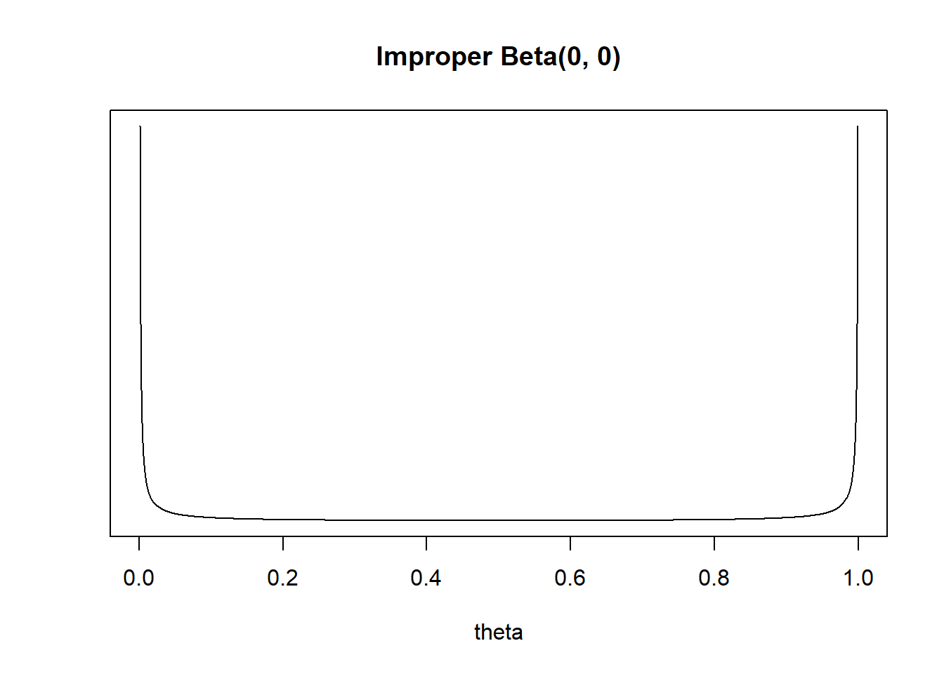
Would you say this is a “noninformative” prior? It seems to concentrate almost all prior “density” near 0 and 1.
Beta(0, 0) is an “improper” prior. It’s not a proper prior distribution, but it can lead to a proper posterior distribution. The likelihood is \(f(y=4|\theta) \propto \theta^4 (1-\theta)^{16}, 0 < \theta < 1\). If we assume the prior is \(\pi(\theta)\propto\theta^{-1}(1-\theta)^{-1}, 0 < \theta <1\), then the posterior is \[ \pi(\theta|y = 4) \propto \left(\theta^{-1}(1-\theta)^{-1}\right)\left(\theta^4 (1-\theta)^{16}\right) = \theta^{4 - 1} (1-\theta)^{16 - 1}, \qquad 0 <\theta < 1 \] That is, the posterior distribution is the Beta(4, 16) distribution. The posterior mean is 4/20=0.2, the sample proportion. Hoever, the posterior mode is \(\frac{4- 1}{4 + 16 -2}= \frac{3}{18} = 0.167\). So the posterior mode does not let the “data speak entirely for itself”.
If \(\theta=0\) then \(\phi=0\); if \(\theta=1\) then \(\phi = \infty\). So \(\phi\) takes values in \((0, \infty)\). We might choose a flat prior on \((0,\infty)\), \(\pi(\phi) \propto 1, \phi > 0\). However, this would be an improper prior.
Simulate a value of \(\theta\) from a Beta(1, 1) distribution, compute \(\phi = \frac{\theta}{1-\theta}\), and repeat many times. The simulation results are below. (The distribution is extremely skewed to the right, so we’re only plotting values in (0, 50).)
```
theta = rbeta(1000000, 1, 1)
odds = theta / (1 - theta)
hist(odds[odds<50], breaks = 100, xlab = "odds", freq = FALSE,
 ylab = "density",
 main = "Prior distribution of odds if prior distribution of probability is Uniform(0, 1)")
```
Even though the prior for \(\theta\) was flat, the prior for a transformation of \(\theta\) is not.

An improper prior distribution is a prior distribution that does not integrate to 1, so is not a proper probability density. However, an improper proper often results in a proper posterior distribution. Thus, improper prior distributions are sometimes used in practice.

Flat priors are common choices in some situations, but are rarely ever the best choices from a modeling perspective. Furthermore, flat priors are generally not preserved under transformations of parameters. So a prior that is flat under one parametrization of the problem will generally not be flat under another. For example, when trying to estimate a population SD \(\sigma\), assuming a flat prior for \(\sigma\) will result in a non-flat prior for the population variance \(\sigma^2\), and vice versa.

Example 9.4 Suppse that \(\theta\) represents the population proportion of adults who have a particular rare disease.

Explain why you might not want to use a flat Uniform(0, 1) prior for \(\theta\).
Assume a Uniform(0, 1) prior. Suppose you will test \(n=100\) suspected cases. Use simulation to approximate the prior predictive distribution of the number in the sample who have the disease. Does this seem reasonable?
Assume a Uniform(0, 1) prior. Suppose that in \(n=100\) suspected cases, none actually has the disease. Find and interpret the posterior median. Does this seem reasonable?

\iffalse{} Solution. to Example 9.4

We know it’s a rare disease! We want to concentrate most of our prior probability for \(\theta\) near 0.
If the disease is rare, we might not expect any actual cases in a sample of 100, maybe 1 or 2. However, the prior predictive distribution says that any value between 0 and 100 actual cases is equally likely! This seems very unreasonable given that the disease is rare.
```
theta_sim = runif(10000)
y_sim = rbinom(10000, 100, theta_sim)
hist(y_sim,
     xlab = "Simulated number of successes",
     main = "Prior predictive distribution")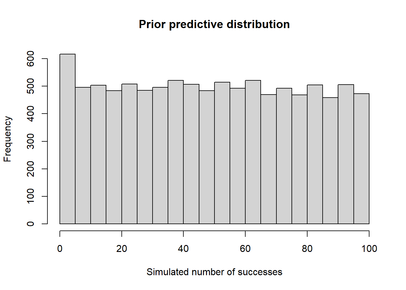
```
The posterior distribution is the Beta(1, 101) distribution. The posterior median is 0.007 (qbeta(0.5, 1, 101)). Based on a sample of 100 suspected cases with no actual cases, there is a posterior probability of 50% that more than 0.7% of people have the disease. A rate of 7 actual cases in 1000 is not a very rare disease, and we think there’s a 50% chance that the rate is even greater than this? Again, this does not seem very reasonable based on our knowledge that the disease is rare.

Prior predictive distributions can be used to check the reasonableness of a prior for a given situation before observing sample data. Do the simulated samples seem consistent with what you might expect of the data based on your background knowledge of the situation? If not, another prior might be more reasonable.