Chapter 6 Introduction to Inference
In a Bayesian analysis, the posterior distribution contains all relevant information about parameters after observing sample data. We can use the posterior distribution to make inferences about parameters.
Example 6.1 Suppose we want to estimate \(\theta\), the population proportion of American adults who have read a book in the last year.
- Sketch your prior distribution for \(\theta\). Make a guess for your prior mode.
- Suppose Henry formulates a Normal distribution prior for \(\theta\). Henry’s prior mean is 0.4 and prior standard deviation is 0.1. What does Henry’s prior say about \(\theta\)?
- Suppose Mudge formulates a Normal distribution prior for \(\theta\). Mudge’s prior mean is 0.4 and prior standard deviation is 0.05. Who has more prior certainty about \(\theta\)? Why?
Show/hide solution
- Your prior distribution is whatever it is and represents your assessment of the degree of uncertainty of \(\theta\).
- The posterior mean, median, and mode are all 0.4. A Normal distribution follows the empirical rule. In particular, the interval [0.3, 0.5] accounts for 68% of prior plausibility, [0.2, 0.6] for 95%, and [0.1, 0.7] for 99.7% of prior plausibility. Henry thinks \(\theta\) is around 0.4, about twice as likely to lie inside the interval [0.3, 0.5] than to lie outside, and he would be pretty surprised if \(\theta\) were outside of [0.1, 0.7].
- Mudge has more prior certainty about \(\theta\) due to the smaller prior standard deviation. The interval [0.3, 0.5] accounts for 95% of Mudge’s plausibility, versus 68% for Henry.
The previous section discussed Bayesian point estimates of parameters, including the posterior mean, median, and mode. In some sense these values provide a single number “best guess” of the value of \(\theta\). However, reducing the posterior distribution to a single-number point estimate loses a lot of the information the posterior distribution provides. In particular, the posterior distribution quantifies the uncertainty about \(\theta\) after observing sample data. The posterior standard deviation summarizes in a single number the degree of uncertainty about \(\theta\) after observing sample data. The smaller the posterior standard deviation, the more certainty we have about the value of the parameter after observing sample data. (Similar considerations apply for the prior distribution. The prior standard deviation summarizes in a single number the degree of uncertainty about \(\theta\) before observing sample data.)
Recall that the variance of a random variable \(U\) is its probability-weighted average squared distance from its expected value \[ \text{Var}(U) = \text{E}\left[\left(U - \text{E}(U)\right)^2\right] \] The following is an equivalent “shortcut” formula for variance: “expected value of the square minus the square of the expected value.” \[ \text{Var}(U) = \text{E}(U^2) - \left(\text{E}(U)\right)^2 \] The standard deviation of a random variable is the square root of its variance is \(\text{SD}(U)=\sqrt{\text{Var}(U)}\). Standard deviation is measured in the same measurement units as the variable itself, while variance is measured in squared units.
In the calculation of a posterior standard deviation, \(\theta\) plays the role of the variable \(U\) and the posterior distribution provides the probability-weights.
Example 6.2 Continuing Example 6.1, we’ll assume a Normal prior distribution for \(\theta\) with prior mean 0.4 and prior standard deviation 0.1.
Compute and interpret the prior probability that \(\theta\) is greater than 0.7.
Find the 25th and 75th percentiles of the prior distribution. What is the prior probability that \(\theta\) lies in the interval with these percentiles as endpoints? According to the prior, how plausible is it for \(\theta\) to lie inside this interval relative to outside it? (Hint: use
qnorm)Repeat the previous part with the 10th and 90th percentiles of the prior distribution.
Repeat the previous part with the 1st and 99th percentiles of the prior distribution.
In a sample of 150 American adults, 75% have read a book in the past year. (The 75% value is motivated by a real sample we’ll see in a later example.)
Find the posterior distribution based on this data, and make a plot of prior, likelihood, and posterior.
Compute the posterior standard deviation. How does it compare to the prior standard deviation? Why?
Compute and interpret the posterior probability that \(\theta\) is greater than 0.7. Compare to the prior probability.
Find the 25th and 75th percentiles of the posterior distribution. What is the posterior probability that \(\theta\) lies in the interval with these percentiles as endpoints? According to the posterior, how plausible is it for \(\theta\) to lie inside this interval relative to outside it? Compare to the prior interval.
Repeat the previous part with the 10th and 90th percentiles of the posterior distribution.
Repeat the previous part with the 1st and 99th percentiles of the posterior distribution.
Show/hide solution
We can use software (
1 - pnorm(0.7, 0.4, 0.1)) but we can also use the empirical rule. For a Normal(0.4, 0.1) distribution, the value 0.7 is \(\frac{0.7-0.4}{0.1} = 3\) SDs above the mean, so the probability is about 0.0015 (since about 99.7% of values are within 3 SDs of the mean). According to the prior, there is about a 0.1% chance that more than 70% of Americans adults have read a book in the last year.We can use
qnorm(0.75)= 0.6745 to find that the 75th percentile of a Normal distribution is about 0.67 SDs above the mean, so the 25th percentile is about 0.67 SDs below the mean. For the prior distribution, the 25th percentile is about 0.33 and the 75th percentile is about 0.47. The prior probability that \(\theta\) lies in the interval [0.33, 0.47] is about 50%. According to the prior, it is equally plausible for \(\theta\) to lie inside the interval [0.33, 0.47] as to lie outside this interval.We can use
qnorm(0.9)= 1.28 to find that the 90th percentile of a Normal distribution is about 1.28 SDs above the mean, so the 10th percentile is about 1.28 SDs below the mean. For the prior distribution, the 10th percentile is about 0.27 and the 90th percentile is about 0.53. The prior probability that \(\theta\) lies in the interval [0.27, 0.53] is about 80%. According to the prior, it is four times more plausible for \(\theta\) to lie inside the interval [0.27, 0.53] than to lie outside this interval.We can use
qnorm(0.99)= 2.33 to find that the 99th percentile of a Normal distribution is about 2.33 SDs above the mean, so the 1st percentile is about 2.33 SDs below the mean. For the prior distribution, the 1st percentile is about 0.167 and the 99th percentile is about 0.633. The prior probability that \(\theta\) lies in the interval [0.167, 0.633] is about 98%. According to the prior, it is 49 times more plausible for \(\theta\) to lie inside the interval [0.167, 0.633] than to lie outside this interval.See below for a plot. Our prior gave very little plausibility to a sample like the one we actually observed. However, given our sample data, the likelihood corresponding to the values of \(\theta\) we initially deemed most plausible is very low. Therefore, our posterior places most of the plausibility on values in the neighborhood of the observed sample proportion, even though the prior probability for many of these values was low. The prior does still have some influence; the posterior mean is 0.709 so we haven’t shifted all the way towards the sample proportion yet.
Compute the posterior variance first using either the definition or the shortcut version, then take the square root; see code below. The posterior SD is 0.036, almost 3 times smaller than the prior SD. After observing data we have more certainty about the value of the parameter, resulting in a smaller posterior SD. The posterior distribution is approximately Normal with posterior mean 0.709 and posterior SD 0.036.
We can use the grid approximation; just sum the posterior probabilities for \(\theta > 0.7\) to see that the posterior probability is about 0.603. Since the posterior distribution is approximately Normal, we can also use the empirical rule: the standardized value for 0.7 is \(\frac{0.7 - 0.709}{0.036}=-0.24\), or 0.24 SDs below the mean. Using the empirical rule (or software
1 - pnorm(-0.24)) gives about 0.596, similar to the grid calculation.We started with a very low prior probability that more than 70% of American adults have read at least one book in the last year. But after observing a sample in which more than 70% have read at least one book in the last year, we assign a much higher plausibility to more than 70% of all American adults having read at least one book in the last year. Seeing is believing.
See code below for calculations based on the grid approximation. But we can also use the fact the posterior distribution is approximately Normal; e.g., the 25th percentile is about 0.67 SDs below the mean: \(0.709 - 0.67 \times 0.036=0.684.\) For the posterior distibution, the 25th percentile is about 0.684 and the 75th percentile is about 0.733. The posterior probability that \(\theta\) lies in the interval [0.684, 0.733] is about 50%. According to the posterior, it is equally plausible for \(\theta\) to lie inside the interval [0.684, 0.733] as to lie outside this interval. This 50% interval is both (1) narrower than the prior interval, due to the smaller posterior SD, and (2) shifted towards higher values of \(\theta\) relative to the prior interval, due to the larger posterior mean.
For the posterior distibution, the 10th percentile is about 0.662 and the 90th percentile is about 0.754. The posterior probability that \(\theta\) lies in the interval [0.662, 0.754] is about 80%. According to the posterior, it is four times more plausible for \(\theta\) to lie inside the interval [0.662, 0.754] as to lie outside this interval. This 80% interval is both (1) narrower than the prior interval, due to the smaller posterior SD, and (2) shifted towards higher values of \(\theta\) relative to the prior interval, due to the larger posterior mean.
For the posterior distibution, the 1st percentile is about 0.622 and the 99th percentile is about 0.789. The posterior probability that \(\theta\) lies in the interval [0.622, 0.789] is about 98%. According to the posterior, it is 49 times more plausible for \(\theta\) to lie inside the interval [0.622, 0.789] as to lie outside this interval. This interval is both (1) narrower than the prior interval, due to the smaller posterior SD, and (2) shifted towards higher values of \(\theta\) relative to the prior interval, due to the larger posterior mean.
theta = seq(0, 1, 0.0001)

# prior
prior = dnorm(theta, 0.4, 0.1) # shape of prior
prior = prior / sum(prior) # scales so that prior sums to 1

# data
n = 150 # sample size
y = round(0.75 * n, 0) # sample count of success

# likelihood, using binomial
likelihood = dbinom(y, n, theta) # function of theta

# posterior
product = likelihood * prior
posterior = product / sum(product)

# posterior mean
posterior_mean = sum(theta * posterior)
posterior_mean
## [1] 0.7024# posterior_variance - "shortcut" formula
posterior_var = sum(theta ^ 2 * posterior) - posterior_mean ^ 2
posterior_sd = sqrt(posterior_var)
posterior_sd## [1] 0.03597# posterior probability that theta is greater than 0.7
sum(posterior[theta > 0.7])## [1] 0.5345# posterior percentiles - central 50% interval
theta[max(which(cumsum(posterior) < 0.25))]## [1] 0.6783theta[max(which(cumsum(posterior) < 0.75))]## [1] 0.727# posterior percentiles - central 80% interval
theta[max(which(cumsum(posterior) < 0.1))]## [1] 0.6557theta[max(which(cumsum(posterior) < 0.9))]## [1] 0.7481# posterior percentiles - central 98% interval
theta[max(which(cumsum(posterior) < 0.01))]## [1] 0.6161theta[max(which(cumsum(posterior) < 0.99))]## [1] 0.7828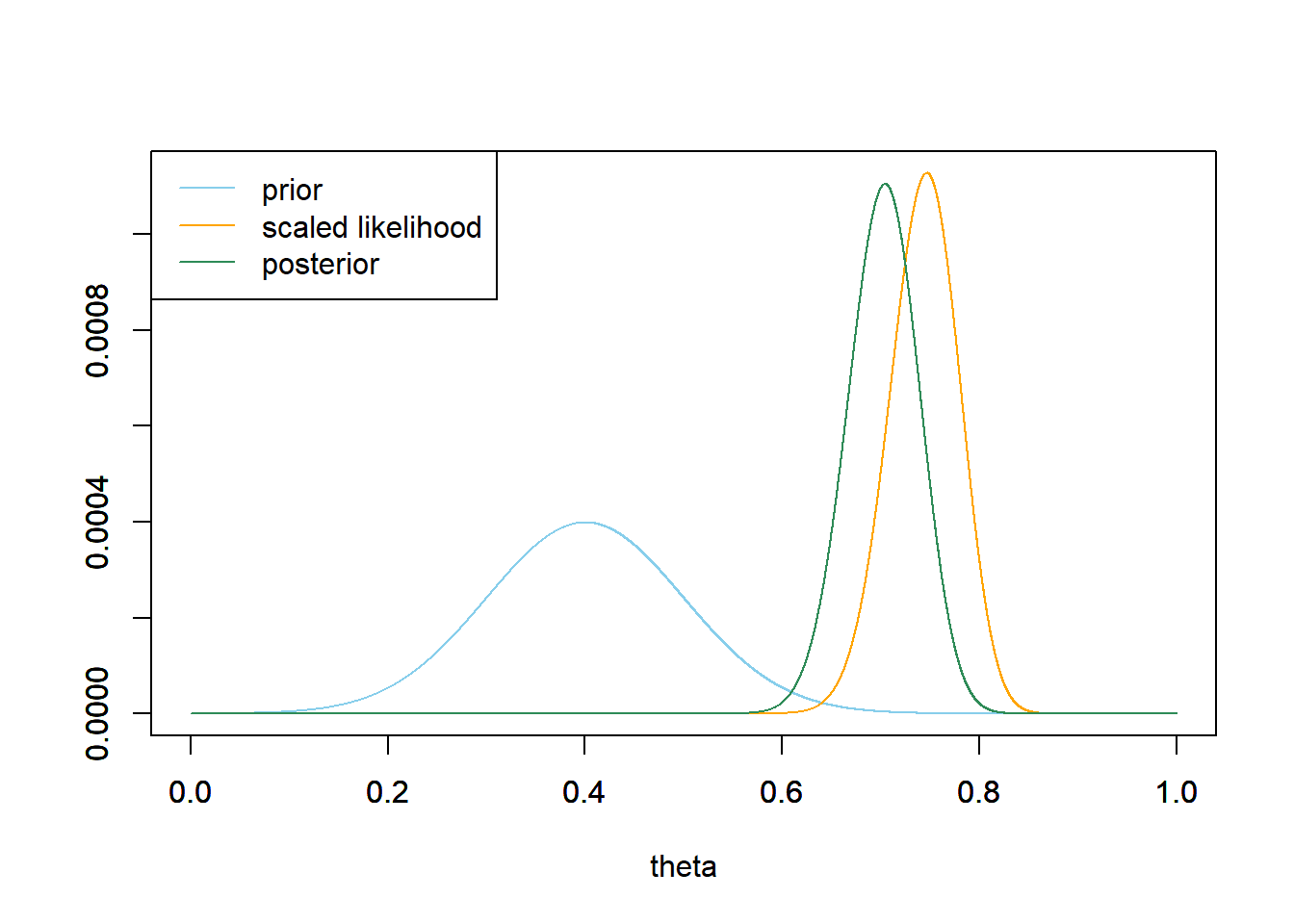
Bayesian inference for a parameter is based on its posterior distribution. Since a Bayesian analysis treats parameters as random variables, it is possible to make probability statements about a parameter.
A Bayesian credible interval is an interval of values for the parameter that has at least the specified probability, e.g., 50%, 80%, 98%. Credible intervals can be computed based on both the prior and the posterior distribution, though we are primarily interested in intervals based on the posterior distribution. For example,
- With a 50% credible interval, it is equally plausible that the parameter lies inside the interval as outside
- With an 80% credible interval, it is 4 times more plausible that the parameter lies inside the interval than outside
- With a 98% credible interval, it is 49 times more plausible that the parameter lies inside the interval than outside
Central credible intervals split the complementary probability evenly between the two tails. For example,
- The endpoints of a 50% central posterior credible interval are the 25th and the 75th percentiles of the posterior distribution.
- The endpoints of an 80% central posterior credible interval are the 10th and the 90th percentiles of the posterior distribution.
- The endpoints of a 98% central posterior credible interval are the 1st and the 99th percentiles of the posterior distribution.
There is nothing special about the values 50%, 80%, 98%. These are just a few convenient choices13 whose endpoints correspond to “round number” percentiles (1st, 10th, 25th, 75th, 90th, 99th) and inside/outside ratios (1-to-1, 4-to-1, about 50-to-1). You could also throw in, say 70% (15th and 85th percentiles, about 2-to-1) or 90% (5th and 95th percentiles, about 10-to-1), if you wanted. As the previous example illustrates, it’s not necessary to just select a single credible interval (e.g., 95%). Bayesian inference is based on the full posterior distribution. Credible intervals simply provide a summary of this distribution. Reporting a few credible intervals, rather than just one, provides a richer picture of how the posterior distribution represents the uncertainty in the parameter.
In many situations, the posterior distribution of a single parameter is approximately Normal, so posterior probabilities can be approximated with Normal distribution calculations — standardizing and using the empirical rule. In particular, an approximate central credible interval has endpoints \[ \text{posterior mean} \pm z^* \times \text{posterior SD} \] where \(z^*\) is the appropriate multiple for a standard Normal distribution corresponding to the specified probability. For example,
| Central credibility | 50% | 80% | 95% | 98% |
|---|---|---|---|---|
| Normal \(z^*\) multiple | 0.67 | 1.28 | 1.96 | 2.33 |
Central credible intervals are easier to compute, but are not the only or most widely used credible intervals. A highest posterior density interval is the interval of values that has the specified posterior probability and is such that the posterior density within the interval is never lower than the posterior density outside the interval. If the posterior distribution is relatively symmetric with a single peak, central posterior credible intervals and highest posterior density intervals are similar.
Example 6.3 Continuing Example 6.1, we’ll assume a Normal prior distribution for \(\theta\) with prior mean 0.4 and prior standard deviation 0.1.
In a recent survey of 1502 American adults conducted by the Pew Research Center, 75% of those surveyed said thay have read a book in the past year.
- Find the posterior distribution based on this data, and make a plot of prior, likelihood, and posterior. Describe the posterior distribution. How does this posterior compare to the one based on the smaller sample size (\(n=150\))?
- Compute and interpret the posterior probability that \(\theta\) is greater than 0.7. Compare to the prior probability.
- Compute and interpret in context 50%, 80%, and 98% central posterior credible intervals.
- Here is how the survey question was worded: “During the past 12 months, about how many BOOKS did you read either all or part of the way through? Please include any print, electronic, or audiobooks you may have read or listened to.” Does this change your conclusions? Explain.
Show/hide solution
See below for code and plots. The posterior distribution is approximately Normal with posterior mean 0.745 and posterior SD 0.011. Despite our prior beliefs that \(\theta\) was in the 0.4 range, enough data has convinced us otherwise. With a large sample size, the prior has little influence on the posterior; much less than with the smaller sample size. Compared to the posterior based on the small sample size, the posterior now (1) has shifted to the neighborhood of the sample data, (2) exhibits a smaller degree of uncertainty about the parameter.
The posterior probability that \(\theta\) is greater than 0.7 is about 0.9999. We started with only a 0.1% chance that more than 70% of American adults have read a book in the last year, but the large sample has convinced us otherwise.
There is a posterior probability of:
- 50% that the population proportion of American adults who have read a book in the past year is between 0.737 and 0.753. We believe that the population proportion is as likely to be inside this interval as outside.
- 80% that the population proportion of American adults who have read a book in the past year is between 0.730 and 0.759. We believe that the population proportion is four times more likely to be inside this interval than to be outside it.
- 98% that the population proportion of American adults who have read a book in the past year is between 0.718 and 0.771. We believe that the population proportion is 49 times more likely to be inside this interval than to be outside it.
In short, our conclusion is that somewhere-in-the-70s percent of American adults have read a book in the past year. But see the next part…
It depends on what our goal is. Do we want to only count completed books? Does there have to be a certain word count? Does it count if the adult read a children’s book? Does listening to an audiobook count? Does it have to be for “fun” or does reading books for work count? If our goal is to estimate the population proportion of Americans who have read completely a 100,000 word non-audiobook book in the last year, then this particular sample data would be fairly biased from our perspective.
theta = seq(0, 1, 0.0001)

# prior
prior = dnorm(theta, 0.4, 0.1) # shape of prior
prior = prior / sum(prior) # scales so that prior sums to 1

# data
n = 1502 # sample size
y = round(0.75 * n, 0) # sample count of success

# likelihood, using binomial
likelihood = dbinom(y, n, theta) # function of theta

# posterior
product = likelihood * prior
posterior = product / sum(product)

# posterior mean
posterior_mean = sum(theta * posterior)
posterior_mean
## [1] 0.745# posterior_variance - "shortcut" formula
posterior_var = sum(theta ^ 2 * posterior) - posterior_mean ^ 2
posterior_sd = sqrt(posterior_var)
posterior_sd## [1] 0.01123# posterior probability that theta is greater than 0.7
sum(posterior[theta > 0.7])## [1] 0.9999# posterior percentiles - central 50% interval
theta[max(which(cumsum(posterior) < 0.25))]## [1] 0.7374theta[max(which(cumsum(posterior) < 0.75))]## [1] 0.7525# posterior percentiles - central 80% interval
theta[max(which(cumsum(posterior) < 0.1))]## [1] 0.7304theta[max(which(cumsum(posterior) < 0.9))]## [1] 0.7592# posterior percentiles - central 98% interval
theta[max(which(cumsum(posterior) < 0.01))]## [1] 0.7183theta[max(which(cumsum(posterior) < 0.99))]## [1] 0.7705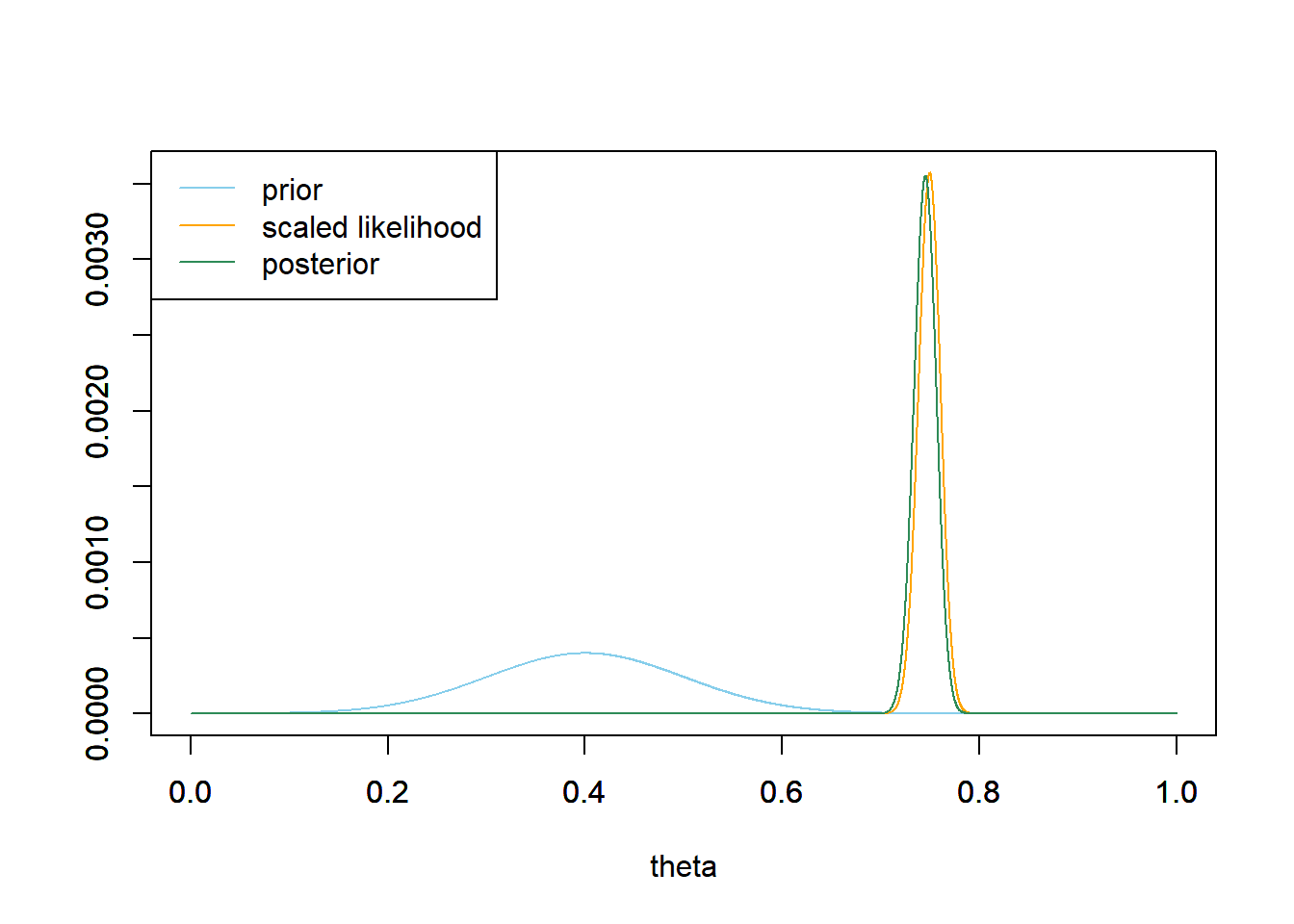
The quality of any statistical analysis depends very heavily on the quality of the data. Always investigate how the data were collected to determine what conclusions are appropriate. Is the sample reasonably representative of the population? Were the variables reliably measured?
Example 6.4 Continuing Example 6.3, we’ll use the same sample data (\(n=1502\), 75%) but now we’ll consider different priors.
For each of the priors below, plot prior, likelihood, and posterior, and compute the posterior probability that \(\theta\) is greater than 0.7. Compare to Example 6.3.
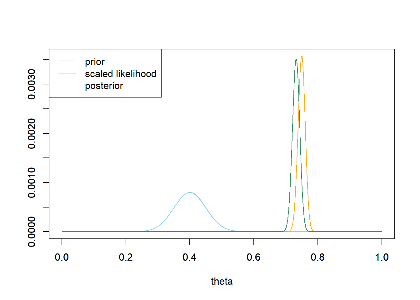
- Normal distribution prior with prior mean 0.4 and prior SD 0.05.
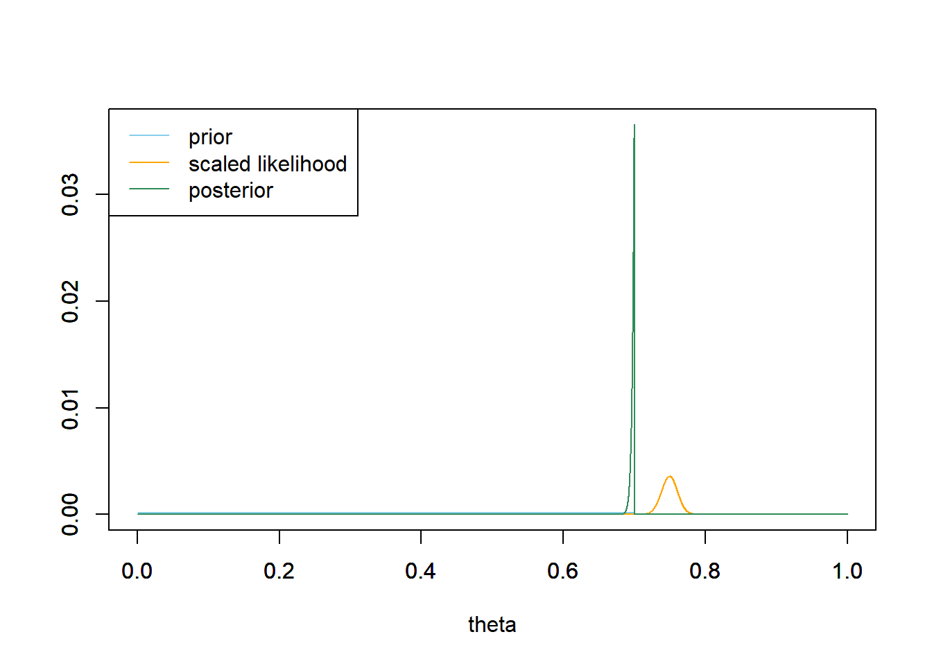
- Uniform distribution prior on the interval [0, 0.7]
Show/hide solution
- The Normal(0.4, 0.05) prior concentrates almost all prior plausibility in a fairly narrow range of values (0.25 to 0.55 or so) and represents more prior certainty about \(\theta\) than the Normal(0.4, 0.1) prior. Even with the large sample size, we see that the Normal(0.4, 0.05) prior has more influence on the posterior than the Normal(0.4, 0.1). However, the two posterior distributions are not that different: Normal(0.73, 0.011) here compared with Normal(0.745, 0.011) from the previous problem. Both posteriors assign almost all posterior credibility to values in the low to mid 70s percent. In particular, the posterior probability that \(\theta\) is greater than 0.7 is 0.997 (compared with 0.9999 from the previous problem).
- The Uniform prior distribution spreads prior plausibility over a fairly wide range of values, [0, 0.7]. However, the prior probability that \(\theta\) is greater than 0.7 is 0. Even when we observed a large sample with a sample proportion greater than 0.7, the posterior probability that \(\theta\) is greater than 0.7 remains 0. See the plot below; the posterior distribution is basically a spike that puts almost all of the posterior credibility on the value 0.7. Assigning 0 prior probability for \(\theta\) values greater than 0.7 has essentially identified such \(\theta\) values as impossible, and no amount of data can make the impossible possible.
You have a great deal of flexibility in choosing a prior, and there are many reasonable approaches. However, do NOT choose a prior that assigns 0 probability/density to possible values of the parameter regardless of how initially implausible the values are. Even very stubborn priors can be overturned with enough data, but no amount of data can turn a prior probability of 0 into a positive posterior probability. Always consider the range of possible values of the parameter, and be sure the prior density is non-zero over the entire range of possible values.