Chapter 18 Some Diagnostics for MCMC Simulation

The goal we wish to achieve with MCMC is to simulate from a probability distribution of interest (e.g., the posterior distribution). The idea of MCMC is to build a Markov chain whose long run distribution is the probability distribution of interest. Then we can simulate a sample from the probability distribution, and use the simulated values to summarize and investigate characteristics of the probability distribution, by running the Markov chain for a sufficiently large number of steps. In practice, we stop the chain after some number of steps; how can we tell if the chain has sufficiently converged?

In this chapter we will introduce some issues to consider in determining if an MCMC algorithm “works”.

Does the algorithm produce samples that are representative of the target distribution of interest?
Are estimates of characteristics of the distribution (e.g. posterior mean, posterior standard deviation, central 98% credible region) based on the simulated Markov chain accurate and stable?
Is the algorithm efficient, in terms of time or computing power required to run?

Example 18.1 Recall Example 17.2 in which we used a Metropolis algorithm to simulate from a Beta(5, 24) distribution. Given current state \(\theta_c\), the proposal was generated from a \(N(\theta_c,\delta)\) distribution, where \(\delta\) was a specified value (determining what constitutes the “neighborhood” in the continuous random walk analog). The algorithm also needs some initial value of \(\theta\) to start with; in Example 17.2 we used an initial value of 0.5. What is the impact of the initial value?

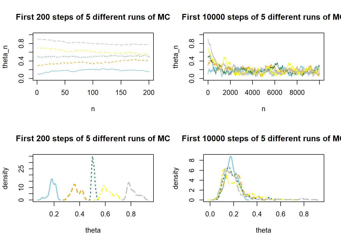
The following plots display the values of the first 200 steps and their density, and the values of 10,000 steps and their density, for 5 different runs of the Metropolis chain each starting from a different initial value: 0.1, 0.3, 0.5, 0.7, 0.9. The value of \(\delta\) is 0.005. (We’re setting this value to be small to illustrate a point.) What do you notice in the plots? How does the initial value influence the results?

\iffalse{} Solution. to Example 18.1

Show/hide solution

With such a small \(\delta\) value the chain tends to take a long time to move away from its current value. For example, the chain that starts at a value of 0.9 tends to stay near 0.9 for the first hundreds of steps. Values near 0.9 are rare in a Beta(5, 24) distribution, so this chain generates a lot of unrepresentative values before it warms up to the target distribution. After a thousand or so iterations all the chains start to overlap and become indistinguishable regardless of the initial condition. However, the density plots for each of the chains illustrate that the initial steps of the chain still carry some influence.

The goal of an MCMC simulation is to simulate a representative sample of values from the target distribution. While an MCMC algorithm should converge eventually to the target distribution, it might take some time to get there. In particular, it might take a while for the influence of the initial state to diminish. Burn in refers to the process of discarding the first several hundred or thousand steps of the chain to allow for a “warm up” period. Only values simulated after the burn in period are used to approximate the target distribution.

The update step in rjags runs the MCMC simulation for a burn in period, consisting of n.iter steps. (The n.iter in update is not the same as the n.iter in coda.samples.) The update function merely “warms-up” the simulation, and the values sampled during the update phase are not recorded.

The JAGS code below simulates 5 different chains, from 5 different initial conditions, each with a burn in period of 1000 steps, after which 10,000 steps of each chain are simulated. The output consists of 50,000 simulated values of \(\theta\).

# Data
n = 25
y = 4

# Model
model_string <- "model{

  # Likelihood
  y ~ dbinom(theta, n)

  # Prior
  theta ~ dbeta(1, 3)
  
}"

data_list = list(y = y, n = n)

# Compile
model <- jags.model(textConnection(model_string), 
                    data = data_list,
                    n.chains = 5)

## Compiling model graph
##    Resolving undeclared variables
##    Allocating nodes
## Graph information:
##    Observed stochastic nodes: 1
##    Unobserved stochastic nodes: 1
##    Total graph size: 5
## 
## Initializing model

# Simulate
update(model, n.iter = 1000, progress.bar = "none")

Nrep = 10000

posterior_sample <- coda.samples(model, 
                                 variable.names = c("theta"), 
                                 n.iter = Nrep,
                                 progress.bar = "none")
summary(posterior_sample)

## 
## Iterations = 2001:12000
## Thinning interval = 1 
## Number of chains = 5 
## Sample size per chain = 10000 
## 
## 1. Empirical mean and standard deviation for each variable,
##    plus standard error of the mean:
## 
##           Mean             SD       Naive SE Time-series SE 
##       0.172972       0.069073       0.000309       0.000426 
## 
## 2. Quantiles for each variable:
## 
##   2.5%    25%    50%    75%  97.5% 
## 0.0609 0.1222 0.1652 0.2158 0.3286

plotPost(posterior_sample)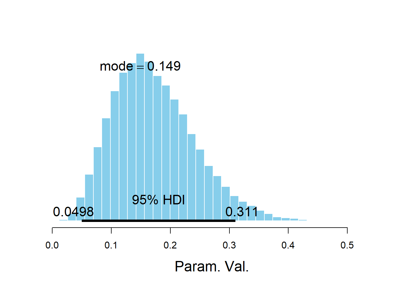

##               ESS  mean median   mode hdiMass  hdiLow hdiHigh compVal
## Param. Val. 26166 0.173 0.1652 0.1491    0.95 0.04979  0.3106      NA
##             pGtCompVal ROPElow ROPEhigh pLtROPE pInROPE pGtROPE
## Param. Val.         NA      NA       NA      NA      NA      NA

nrow(as.matrix(posterior_sample))

## [1] 50000

In practice, it is common to use a burn in period of several hundred or thousands of steps. To get a better idea of how long the burn in period should be, run the chain starting from several disperse initial conditions to see how long it takes for the paths to “overlap”. JAGS will generate different initial values, but you can also specify them with the inits argument in jags.model. After the burn in period, examine trace plots or density plots for multiple chains; if the plots do not “overlap” then there is evidence that the chains have not converged, so they might not be producing representative samples from the target distribution, and therefore a longer burn in period is needed.

The Gelman-Rubin statistic (a.k.a., shrink factor) is a numerical check of convergence based on a measure of variance between chains relative to variability with chains. The idea is that if multiple chains have settled into representative sampling, then the average difference between chains should be equal to the average difference within chains (i.e., across steps). Roughly, if multiple chains are all producing representative samples from the target distribution, then given a current value, it shouldn’t matter if you take the next value from the chain or if you hop to another chain. Thus, after the burn-in period, the shrink factor should be close to 1. As a rule of thumb, a shrink factor above 1.1 is evidence that the MCMC algorithm is not producing representative samples.

Recall that there are several packages available for summarizing MCMC output, and these packages contain various diagnostics. For example, the output of the diagMCMC function in the DBDA2E-utilities.R file includes a plot the shrink factor.

diagMCMC(posterior_sample)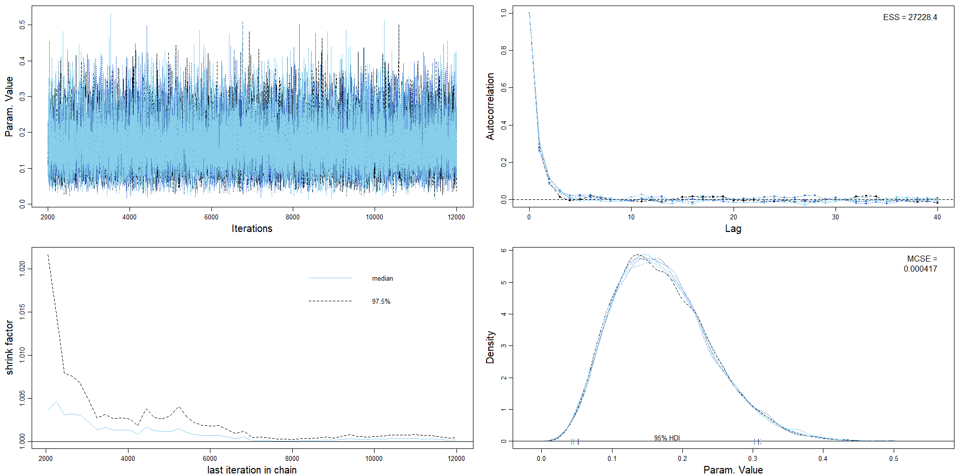

Example 18.2 Continuing with Metropolis sampling from a Beta(5, 24) distribution, the following plots display the results of three different runs, one each for \(\delta=0.01\), \(\delta=0.1\), \(\delta=1\), all with an initial value of 0.5. Describe the differences in the behavior of the chains. Which chain seems “best”? Why?

\iffalse{} Solution. to Example 18.2

Show/hide solution

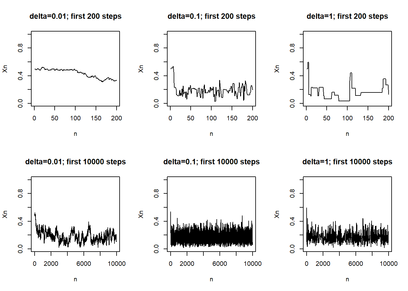
When \(\delta=0.01\) only values that are close to the current value are proposed. A proposed value close to the current value will have a density that is close to, if not greater, than that of the current value. Therefore, most of the proposals will be accepted, but these proposals don’t really go anywhere. With \(\delta=0.01\) the chain moves often, but it does not move far.

When \(\delta=1\) a wide range of values will be proposed, including values outside of (0, 1). Many proposed values will have density that is much less than that of the current value, if not 0. Therefore many proposals will be rejected. With \(\delta=1\) the chain tends to get stuck in a value for a large number of steps before moving (though when it does move, it can move far.)

Both of the above cases tend to get stuck in place and require a large number of steps to explore the target distribution. The case \(\delta=0.1\) is a more efficient. The proposals are neither so narrow that it takes a long time to move nor so wide that many proposals are rejected. The fast up and down pattern of the trace plot shows that the chain with \(\delta=0.2\) explores the target distribution much more efficiently than the other two cases.

The values of a Markov chain at different steps are dependent. If the degree of dependence is too high, the chain will tend to get “stuck”, requiring a large number of steps to fully explore the target distribution of interest. Not only will the algorithm be inefficient, but it can also produce inaccurate and unstable estimates of chararcteristics of the target distribution.

If the MCMC algorithm is working, trace plots should look like a “fat, hairy catepillar.”³⁵ Plots of the autocorrelation function (ACF) can also help determine how “clumpy” the chain is. An autocorrelation measures the correlation between values at different lags. For example, the lag 1 autocorrelation measures the correlation between the values and the values from the next step; the lag 2 autocorrelation measures the correlation between the values and the values from 2 steps later.

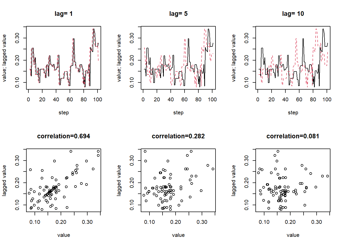
Example 18.3 Continuing with Metropolis sampling from a Beta(5, 24) distribution, the following plots display, for the case \(\delta=0.1\), the actual values of the chain (after burn in) and the values lagged by 1, 5, and 10 time steps. Are the values at different steps dependent? In what way are they not too dependent?

\iffalse{} Solution. to Example 18.3

Show/hide solution

Yes, the values are dependent. In particular, the lag 1 autocorrelation is about 0.8, and the lag 5 autocorrelation is about 0.4. However, the autocorrelation decays rather quickly as a function of lag. The lag 10 autocorrelation is already close to 0. In this way, the chain is “not too dependent”; each value is only correlated with the values in the next few steps.

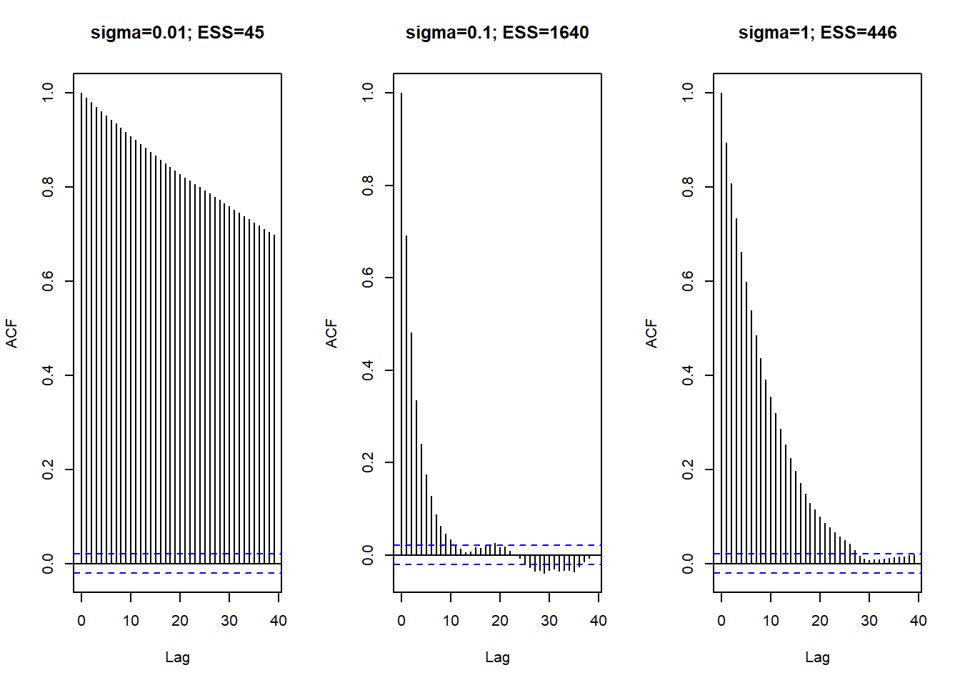
An autocorrelation plot displays the autocorrelation within in a chain as a function of lag. If the ACF takes too long to decay to 0, the chain exhibits a high degree of dependence and will tend to get stuck in place.

The plot below displays the ACFs corresponding to each of the \(\delta\) values in Example 18.2. Notice that with \(\delta=0.2\) the ACF decays fairly quickly to 0, while in the other cases there is still fairly high autocorrelation even after long lags.

Example 18.4 Continuing with Metropolis sampling from a Beta(5, 24) posterior distribution. We know that the posterior mean is \(5/29=0.172\). But what if we want to approximate this via simulation?

Suppose you simulated 10000 independent values from a Beta(5, 24) distribution, e.g. using rbeta. How would you use the simulated values to estimate the posterior mean?
What is the standard error of your estimate from the previous part? What does the standard error measure? How could you use simulation to approximate the standard error?
Now suppose you simulated 10000 from a Metropolis chain (after burn in). How would you use the simulated values to estimate the posterior mean? What does the standard error measure in this case? Could you use the formula from the previous part to compute the standard error? Why?
Consider the three chains in Example 18.2 corresponding to the three \(\delta\) values 0.01, 0.1, and 1. Which chain provides the most reliable estimate of the posterior mean? Which chain yields the smallest standard error of this estimate?

\iffalse{} Solution. to Example 18.4

Show/hide solution

Simulate 10000 values and compute the sample mean of the simulated values.
For the Beta(5, 24) distribution, the population SD is \(\sqrt{(5/29)(1-5/29)/(29+1)} = 0.07\). The standard error of the sample mean of 10000 values is \(0.07/\sqrt{10000} = 0.0007\). The standard error measures the sample-to-sample variability of sample means over many samples of size 10000. To approximate the standard error via simulation: sample 10000 values from a Beta(5, 24) distribution and compute the sample mean, then repeat many times and find the standard deviation of the simulated sample means.
You would still use the sample mean of the 10000 values to approximate the posterior mean. The standard error measures how much the sample mean varies from run-to-run of the Markov chain. To approximate the standard error via simulation: simulate 10000 steps of the Metropolis chain and compute the sample mean, then repeat many times and find the standard deviation of the simulated sample means. The standard error formula from the previous part assumes that the 10000 values are independent, but the values on the Markov chain are not, so we can’t use the same formula.
Among these three, the chain with \(\delta=0.1\) provides the most reliable estimate of the posterior mean since it does the best job of sampling from the posterior distribution. While there is dependence in all three chains, the chain with \(\delta=0.1\) has the least dependence and so comes closest to independent sampling, so it would have the smallest standard error.

A Markov chain that exhibits a high degree of dependence will tend to get stuck in place. Even if you simulate 10000 steps of the chain, you don’t really get 10000 “new” values. The effective sample size (ESS) is a measure of how much independent information there is in an autocorrelated chain. Roughly, the effective sample size answers the question: what is the equivalent sample size of a completely independent chain?

The effective sample size³⁶ of a chain with \(N\) steps (after burn in) is \[ \text{ESS} = \frac{N}{1+2\sum_{\ell=1}^\infty \text{ACF}(\ell)} \] where the infinite sum is typically cut off at some upper lag (say \(\ell=20\)). For a completely independent chain, the autocorrelation would be 0 for all lags and the ESS would just be the number of steps \(N\). The more quickly the ACF decays to 0, the larger the ESS. The more slowly the ACF decays to 0, the smaller the ESS.

The larger the ESS of a Markov chain, the more accurate and stable are MCMC-based estimates of characteristics of the posterior distribution (e.g., posterior mean, posterior standard deviation, 98% credible region). That is, if the ESS is large and we run the chain multiple times, then estimates do not vary much from run to run.

The standard error of a statistic is a measure of its accuracy. The standard error of a statistic measures the sample-to-sample variability of values of the statistic over many samples of the same size. A standard error can be approximated via simulation.

Simulate a sample and compute the value of the statistic.
Repeat many times and find the standard deviation of simulated values of the statistic.

For many statistics (means, proportions) the standard error based on a sample of \(n\) independent values is on the order of \(\frac{1}{\sqrt{n}}\).

For example, the standard error of a sample mean measures the sample-to-sample variability of sample means over many samples of the same size. The standard error of a sample mean based on an independent sample of size \(n\) is \[ \frac{\text{population SD}}{\sqrt{n}} \] where the population SD measures the variability of individual values of the variable.

The usual \(\frac{1}{\sqrt{n}}\) formulas for standard errors are based on samples of \(n\) independent values. However, in a Markov chain the values will be dependent. The Monte Carlo standard error (MCSE) is the standard error of a statistic generated based on an MCMC algorithm. The MCSE of a statistic measures the run-to-run variability of values of the statistic over many runs of the chain of the same number of steps. A MCSE can be approximated via simulation

Simulate many steps of the Markov chain and compute the value of the statistic for the simulated chain
Repeat many times and find the standard deviation of simulated values of the statistic

For many statistics (means, proportions) the MCSE based on a chain with effective sample size ESS is on the order of \(\frac{1}{\sqrt{\text{ESS}}}\).

The MCSE effects the accuracy of parameter estimates based on the MCMC method. If the chain is too dependent, the ESS will be small, the MCSE will be large, and resulting estimates will not be accurate. That is, two different runs of the chain could produce very different estimates of a particular characteristic of the target distribution.

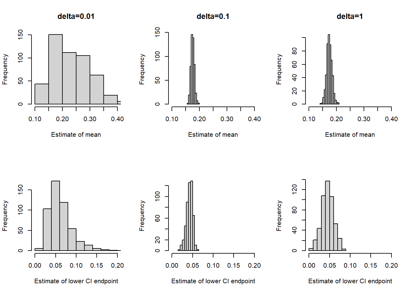
How large of an ESS is appropriate depends on the particular characteristic of the posterior distribution being estimated. A larger ESS will be required for accurate estimates of characteristics that depend heavily on sparse regions of the posterior that are visited relatively rarely by the chain, like the endpoints of a 98% credible interval.

The plot belows correspond to each of the \(\delta\) values in Example 18.2. Each plot represents 500 runs of the chain, each run with 1000 steps (after burn in). For each run we computed both the sample mean (our estimate of the posterior mean) and the 0.5th percentile (our estimate of the lower endpoint of a central 99% credible interval.) Therefore, each plot in the top row displays 500 simulated sample means, and each plot in the bottom row displays 500 simulated 0.5th percentiles. The MCSE is represented by the degree of variability in each plot. We see that for both statistics the MCSE is smallest when \(\delta=0.1\), corresponding to the smallest degree of autocorrelation and the largest ESS.

For most of the situations we’ll see in this course, standard MCMC algorithms will run fairly efficiently, and checking diagnostics is simply a matter of due diligence. However, especially in more complex models, diagnostic checking is an important step in Bayesian data analysis. Poor diagnostics can indicate the need for better MCMC algorithms to obtain a more accurate picture of the posterior distribtuion. Algorithms that use “smarter” proposals will usually lead to better results.