Chapter 19 Introduction to Hierarchical Models

In a Bayesian hierarchical model, the model for the data depends on certain parameters, and those parameters in turn depend on other parameters. Hierarchical modeling provides a framework for building complex and high-dimensional models from simple and low-dimensional building blocks.

Suppose we want to estimate the probability that each basketball player on the Houston Rockets successfully makes a free throw attempt. (That is, we want to estimate each player’s true free throw percentage.) We’ll consider free throw data from the 2018-2019 NBA season for players on the Houston Rockets at the time³⁷.

data = read.csv('_data/rockets.csv')
data = data[order(data$FTA), ] # sort by number of attempts

player = data$Name
y = data$FT
n = data$FTA
J = length(y)

player_summary = data.frame(player, n, y, y / n)
names(player_summary) = c("player", "FTA", "FT", "FTpct")
knitr::kable(player_summary, digits = 3)

player	FTA	FT	FTpct
James Nunnally	0	0	NaN
Iman Shumpert	0	0	NaN
Vince Edwards	0	0	NaN
Zhou Qi	0	0	NaN
Gary Clark	6	6	1.000
Marquese Chriss	7	6	0.857
Brandon Knight	11	9	0.818
Isaiah Hartenstein	14	11	0.786
Carmelo Anthony	22	15	0.682
Austin Rivers	26	14	0.538
Michael Carter-Williams	26	12	0.462
Nene Hilario	31	22	0.710
Kenneth Faried	44	24	0.545
Gerald Green	49	39	0.796
P.J. Tucker	51	33	0.647
Danuel House	55	45	0.818
James Ennis	58	42	0.724
Eric Gordon	118	93	0.788
Chris Paul	121	100	0.826
Clint Capela	174	109	0.626
James Harden	609	529	0.869

Over the 21 players in the data, there are 1422 attempts, of which 1109 were successful, for an overall free throw percentage of 0.78. The sample mean free throw percentage is 0.735.

Let \(\theta_j\) denote the true (long run) probability that player \(j\) successfully make a free throw attempt; for example, \(\theta_{\text{Harden}}\), \(\theta_{\text{Capela}}\), etc. Let \(n_j\) denote the number of free throw attempts and \(y_j\) the number of free throws made for player \(j\).

Example 19.1 We could assume a model with a prior in which all \(\theta_j\) are independent. What are some disadvantages of this model? In particular, what would be an issue for players like James Nunnally?

\iffalse{} Solution. to Example 19.1

Given the parameters \(\theta_j\), it is reasonable to assume that the \(y_j\) are independent across players. Assuming independence in the data, if the \(\theta_j\) are independent in the prior, then the \(\theta_j\) will be independent in the posterior. The posterior distribution of each parameter \(\theta_j\) could be updated separately as in a one-parameter problem, with the posterior distribution of \(\theta_j\) for player \(j\) will be based only on the data \((y_j, n_j)\) for player \(j\). Therefore, we would not be able to find the posterior distribution of \(\theta_j\) for players like James Nunnally with 0 attempts (no data). It would be useful if we could borrow information from other players to estimate free throw percentages for players with few or no attempts.

As we’ve mentioned before, it is often useful to have dependence between parameters. We will introduce a hierarchical model for introducing dependence.

Example 19.2 Let’s first consider just a single player with true free throw percentage \(\theta\). Given \(n\) independent attempts, conditional on \(\theta\), we might assume \((y|\theta)\sim\) Binomial(\(n, \theta\)).

If we imagine the player is randomly selected, how might we interpret the prior distribution for \(\theta\)?
The prior distribution for \(\theta\) has a prior mean \(\mu\). How might we interpret \(\mu\)?
The prior mean \(\mu\) is also a parameter, so we could place a prior distribution on it. What would the prior distribution on \(\mu\) represent?
In this model \(\mu\) and \(\theta\) are dependent. Why is this dependence useful?

\iffalse{} Solution. to Example 19.2

Free throw percentages vary from player to player. There is a distribution of free throw percentages over many players in the league. If the player is randomly selected we can think of the prior distribution \(\pi(\theta)\) as the league-wide distribution of free throw percentages. (This interpretation is kind of mixing Bayesian and frequentist ideas, but I think it helps the motivation.)
With the above interpretation \(\mu\) represents the league-wide average free throw percentage over all players in the league.
We can specify a prior distribution on \(\mu\) to encapsulate our uncertainty in the true league-wide average free throw percentage. For example, if our prior belief is that \(\mu\) is around 0.75 we could choose a prior distribution for \(\mu\) that has a mean (or mode) of 0.75.
When we observe data for a single player, we can directly make inference about \(\theta\) for that player. But since \(\theta\) and \(\mu\) are dependent, we can also use the data for a single player to make inference about the league-wide average. This in turn allows us to use data for a single player to inform inference about other players. We’ll see that this is one of the benefits of a hierarchical model.

In the model in the previous example

The prior distribution on the model parameter \(\theta\) reflects our uncertainty in the individual player’s free throw percentage.
The prior distribution on the hyperparameter \(\mu\) reflects our uncertainty about the league-wide average free throw percentage.

We could translate the setup from the previous example, for a single player, into a Bayesian hierarchical model as follows.

Likelihood. \((y|\theta)\sim\) Binomial(\(n, \theta\)). The likelihood assumes³⁸, conditional on \(\theta\), \(n\) independent attempts with constant probability \(\theta\).
Prior. \((\theta|\mu,\kappa)\sim\) Beta\((\mu\kappa, (1-\mu)\kappa)\).
- The prior distribution for \(\theta\) has two hyperparameters: \(\mu\), \(\kappa\). These parameters represent our prior beliefs about \(\theta\), the free throw percentage of an individual player.
- We might consider \(\theta\sim\) Beta(\(\alpha, \beta\)).
- However, it is often more convenient to reparemetrize a Beta distribution in terms of its mean \(\mu=\alpha/(\alpha+\beta)\) and concentration \(\kappa=\alpha+\beta\) rather than \(\alpha\) and \(\beta\), which is what we’ve done here. So \(\alpha=\mu\kappa\) and \(\beta=(1-\mu)\kappa\).
- \(\mu\) represents what we expect \(\theta\) to be around.
- \(\kappa\) represents the “equivalent prior sample size” upon which our expectations for \(\theta\) are based; larger \(\kappa\) corresponds to stronger prior beliefs about \(\theta\). (Alternatively, \(\kappa\) is inversely related to the variance of the prior distribution, so the larger the \(\kappa\) the smaller the prior variance of \(\theta\) and the closer we expect \(\theta\) to be to \(\mu\).)
Hyperprior. \(\mu, \kappa\) independent with \(\mu\sim\) Beta(15, 5) and \(\kappa\sim\) Gamma\((1, 0.1)\).
- \(\mu\) is the mean of the prior distribution of \(\theta\), which is like the league-wide average free throw percentage. The prior distribution for \(\mu\) represents our uncertainty in the league-wide average free throw percentage. Assuming a Beta(15, 5) prior for \(\mu\) says we expect that the league-wide average free throw percentage is around 0.75, but there is still some uncertainty: 95% prior credible interval for \(\mu\), the league-wide average, is (0.544, 0.909).
- \(\kappa\) represents the “equivalent prior sample size³⁹” upon which our beliefs about \(\theta\) are based. Putting a prior on \(\kappa\) is like allowing for different degrees of strength for our prior beliefs about \(\theta\). (Alternatively, \(\kappa\) is inversely related to the variance of the prior distribution. So putting a prior on \(\kappa\) represents our uncertainty in the league-wide player-to-player variance in free throw percentages.) A Gamma(1, 0.1) prior⁴⁰ has mean 10 and standard deviation 10. So we’re saying our prior beliefs about \(\theta\) are likely based on an “equivalent prior sample size” in the single digits or a few tens (but not hundreds or thousands) of pseudo-observations. This is like saying we haven’t observed any players, so we don’t have much information about the league-wide distribution or player-to-player variability of free throw percentages.

To emphasize:

The prior distribution on \(\theta\) reflects our uncertainty in an individual player’s free throw percentage.
The prior distributions on \(\mu\) and \(\kappa\) reflect our uncertainty about the league-wide player-to-player distribution of free throw percentages.

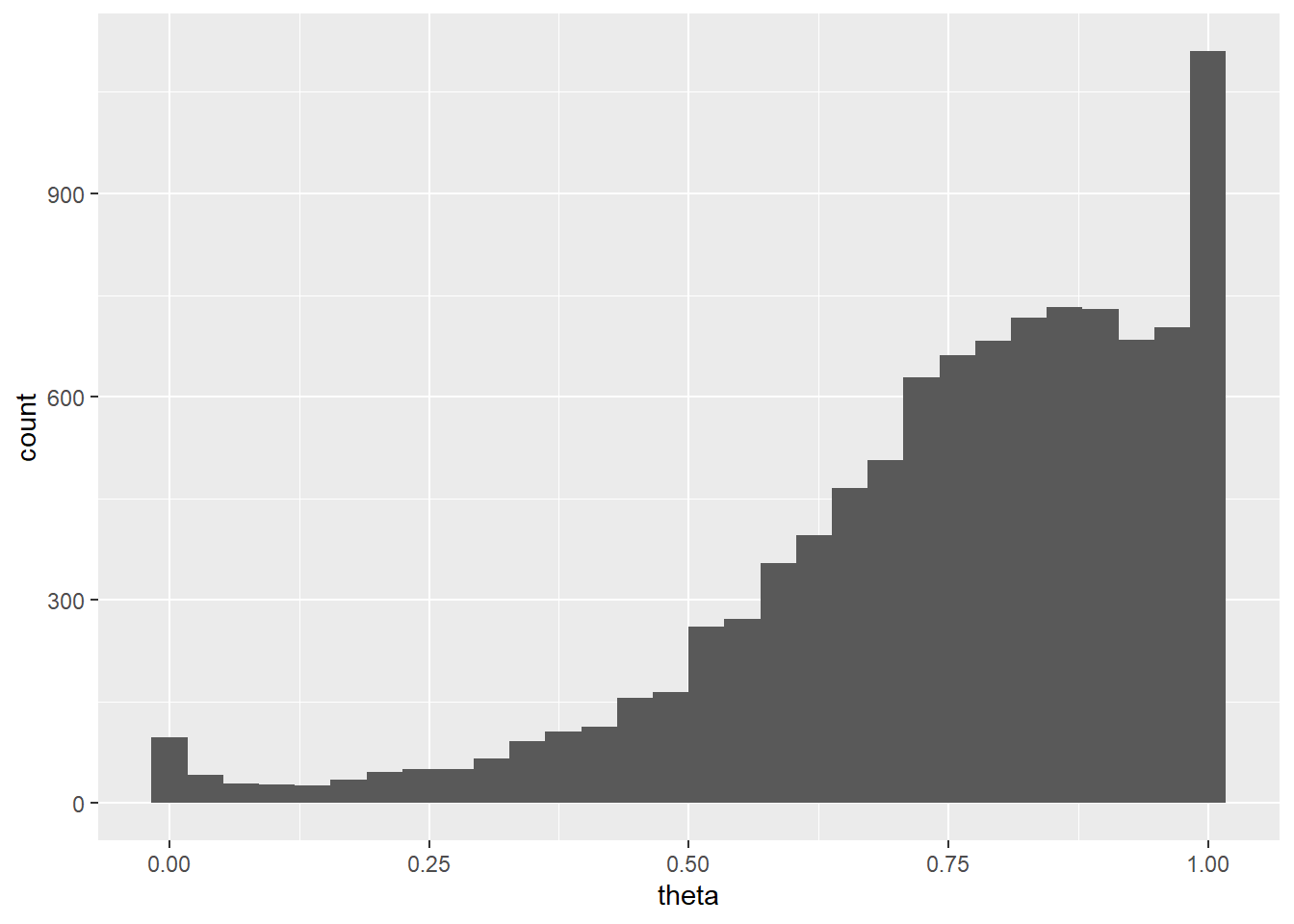
Remember that the posterior distribution is what’s important, but let’s first take a brief look at the prior. Notice the positive correlation between \(\mu\) and \(\theta\). Also notice that while conditional on \(\mu\) and \(\kappa\) the prior distribution of \(\theta\) is a Beta distribution, the marginal prior distribution of \(\theta\) is not a Beta distribution.

N = 10000

# hyperprior
mu = rbeta(N, 15, 5)
kappa = rgamma(N, 1, 0.1)

# prior
theta = rbeta(N, mu * kappa, (1 - mu) * kappa)

sim_prior = data.frame(mu, kappa, theta)

ggplot(sim_prior, aes(mu, theta)) +
  geom_point(color = "skyblue", alpha = 0.4) +
  geom_density_2d(color = "orange", size = 1) +
  geom_abline(intercept = 0, slope = 1, color="black", 
                 linetype="dashed")

cor(mu, theta)

## [1] 0.4395

ggplot(sim_prior, aes(theta)) +
  geom_histogram()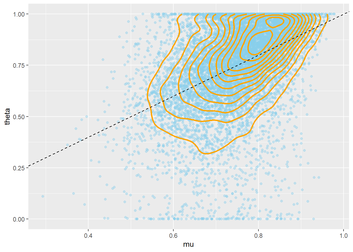

Now suppose we have data on a single player who made \(y=9\) free throws out of \(n=10\) attempts. The following is the JAGS code for approximating the posterior distribution. Note that the hyperprior is specified similarly to the prior. The JAGS output can be used to make posterior inference about the player’s free throw percentage \(\theta\) and the league-wide average free throw percentage.

This example merely motivates the hierarchical model and illustrates the JAGS code. Next we’ll find the posterior distribution based on the Rockets data and inspect it more carefully.

# load the data
y = 9
n = 10

# specify the model: likelihood, prior, hyperprior

model_string <- "model{

  # Likelihood
  y ~ dbinom(theta, n)

  # Prior
  theta ~ dbeta(mu * kappa, (1 - mu) * kappa)
  
  # Hyperprior, phi=(mu, kappa)
  mu ~ dbeta(15, 5)
  kappa ~ dgamma(1, 0.1)
}"

dataList = list(y = y,
                n = n)

model <- jags.model(file = textConnection(model_string), 
                    data = dataList)

## Compiling model graph
##    Resolving undeclared variables
##    Allocating nodes
## Graph information:
##    Observed stochastic nodes: 1
##    Unobserved stochastic nodes: 3
##    Total graph size: 12
## 
## Initializing model

update(model, n.iter = 1000)

posterior_sample <- coda.samples(model,
                       variable.names = c("theta", "mu", "kappa"),
                       n.iter = 10000,
                       n.chains = 5)

summary(posterior_sample)

## 
## Iterations = 2001:12000
## Thinning interval = 1 
## Number of chains = 1 
## Sample size per chain = 10000 
## 
## 1. Empirical mean and standard deviation for each variable,
##    plus standard error of the mean:
## 
##         Mean      SD Naive SE Time-series SE
## kappa 11.602 10.5786 0.105786        0.23989
## mu     0.774  0.0823 0.000823        0.00133
## theta  0.846  0.0919 0.000919        0.00172
## 
## 2. Quantiles for each variable:
## 
##        2.5%   25%   50%    75%  97.5%
## kappa 0.790 4.091 8.513 15.572 40.082
## mu    0.597 0.723 0.784  0.836  0.908
## theta 0.632 0.789 0.859  0.915  0.981

plot(posterior_sample)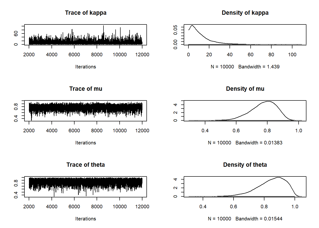

posterior_sample_values = as.matrix(posterior_sample)
theta = posterior_sample_values[, "theta"]
mu = posterior_sample_values[, "mu"]
kappa = posterior_sample_values[, "kappa"]
plotPost(theta, main = "theta")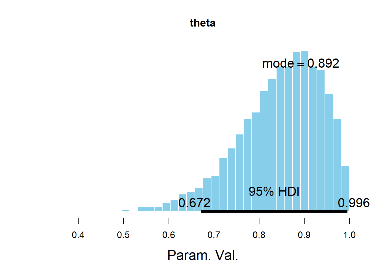

##              ESS   mean median   mode hdiMass hdiLow hdiHigh compVal pGtCompVal
## Param. Val. 2857 0.8457 0.8592 0.8921    0.95 0.6715  0.9956      NA         NA
##             ROPElow ROPEhigh pLtROPE pInROPE pGtROPE
## Param. Val.      NA       NA      NA      NA      NA

plotPost(mu, main = "mu")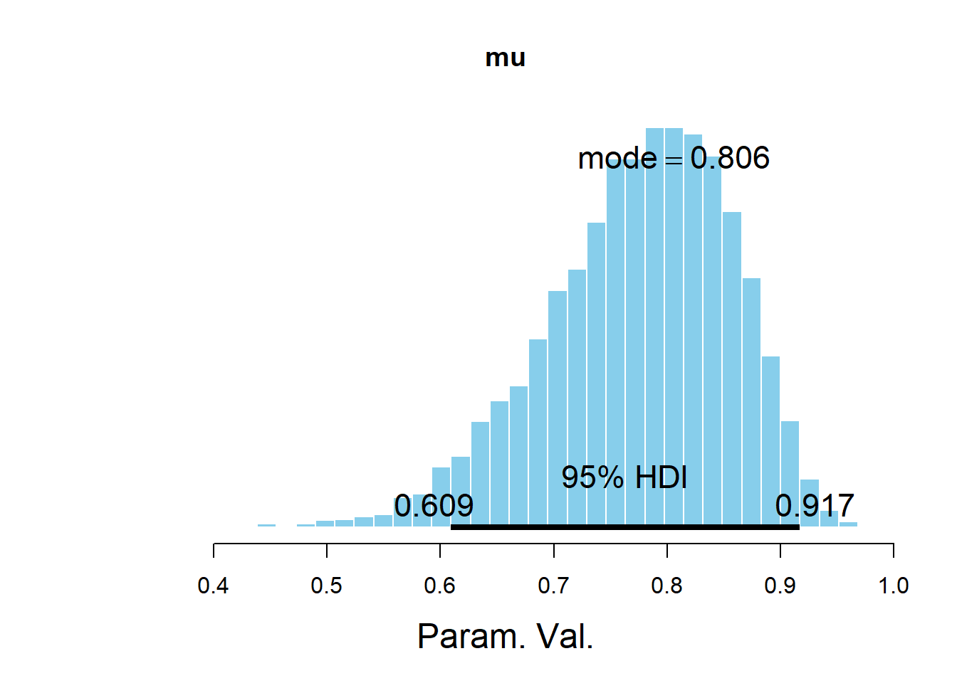

##              ESS   mean median   mode hdiMass hdiLow hdiHigh compVal pGtCompVal
## Param. Val. 3825 0.7744 0.7837 0.8062    0.95  0.609  0.9167      NA         NA
##             ROPElow ROPEhigh pLtROPE pInROPE pGtROPE
## Param. Val.      NA       NA      NA      NA      NA

plotPost(kappa, main = "kappa")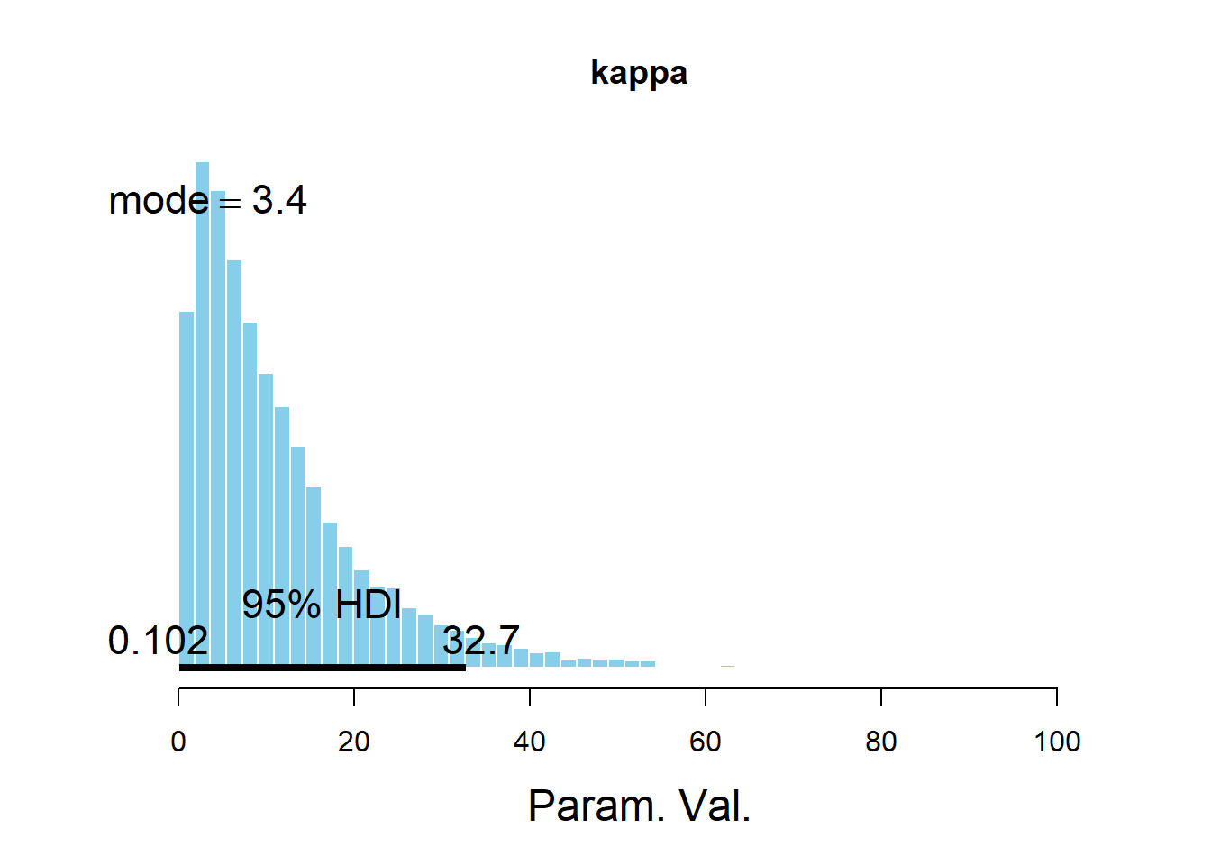

##              ESS mean median  mode hdiMass hdiLow hdiHigh compVal pGtCompVal
## Param. Val. 1945 11.6  8.513 3.401    0.95 0.1023   32.69      NA         NA
##             ROPElow ROPEhigh pLtROPE pInROPE pGtROPE
## Param. Val.      NA       NA      NA      NA      NA

sim_posterior = as.data.frame(posterior_sample_values)

ggplot(sim_posterior, aes(mu, theta)) +
  geom_point(color = "skyblue", alpha = 0.4) +
  geom_density_2d(color = "orange", size = 1) +
  geom_abline(intercept = 0, slope = 1, color="black", 
                 linetype="dashed")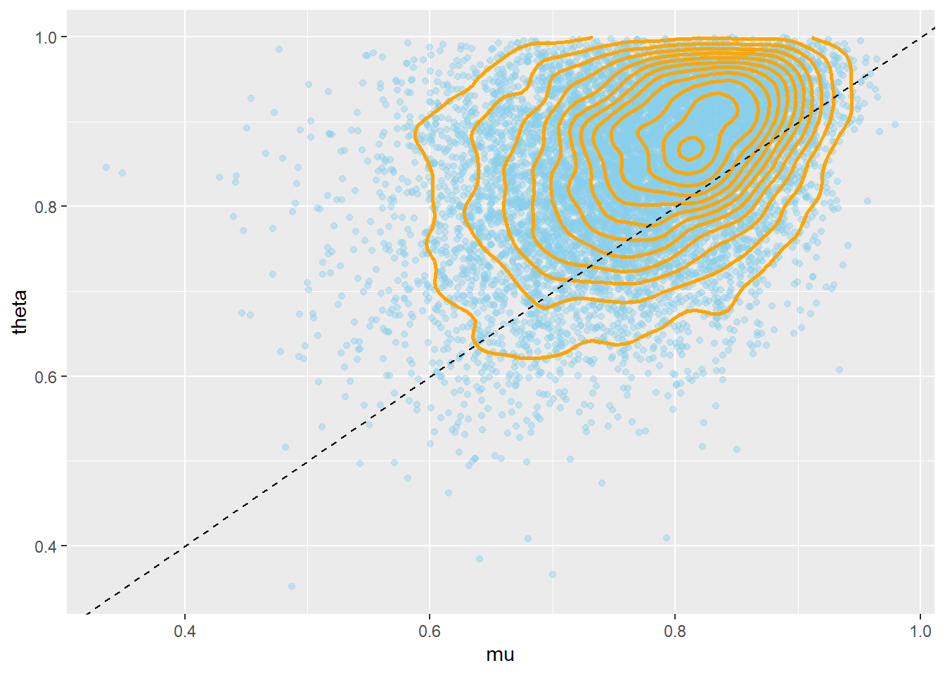

cor(mu, theta)

## [1] 0.3491

A Bayesian hierarchical model consists of the following layers in the hierarchy.

A model for the data \(y\) which depends on model parameters \(\theta\) and is represented by the likelihood \(f(y|\theta)\).
- The model often involves multiple parameters. Generically, \(\theta\) represents a vector of parameters that show up in the likelihood function. (In particular problems, we might use other notation, e.g. \(\theta\) replaced by \((\mu, \sigma)\) when the data are assumed to follow a Normal distribution.)
- Remember: While the likelihood for a particular \((y, \theta)\) value is computed by evaulating the conditional density of \(y\) given \(\theta\), the likelihood function is a function of \(\theta\), treating the data \(y\) as fixed.
A (joint) prior distribution for the model⁴¹ parameter(s) \(\theta\), denoted \(\pi(\theta|\phi)\), which depends on hyperparameters \(\phi\).
A hyperprior distribution, i.e. a prior distribution for the hyperparameters, denoted \(\pi(\phi)\). (Again, \(\phi\) generically represents a vector of hyperparameters.)

The above specification implicitly assumes that the data distribution and likelihood function only depend on \(\theta\); the hyperparameters only affect \(y\) through \(\theta\). That is, the general hierarchical model above assumes that the data \(y\) and hyperparameters \(\phi\) are conditionally independent given the model parameters \(\theta\), so the likelihood satisfies \[ f(y|\theta, \phi) = f(y|\theta) \] The joint prior distribution on parameters and hyperparameters is \[ \pi(\theta, \phi) = \pi(\theta|\phi)\pi(\phi) \]

Given the observed data \(y\), we find the joint posterior density of the parameters and hyperparameters, denoted \(\pi(\theta, \phi|y)\), using Bayes rule: posterior \(\propto\) likelihood \(\times\) prior. \[\begin{align*} \pi(\theta, \phi|y) & \propto f(y|\theta, \phi)\pi(\theta, \phi)\\ & \propto f(y|\theta)\pi(\theta|\phi)\pi(\phi) \end{align*}\]

In Bayesian hierarchical models, there will generally be dependence between parameters. But dependence among parameters is actually useful for several reasons:

The dependence is natural and meaningful in the problem context. For example, we might expect the free throw percentages of guards to be close together.
If parameters are dependendent, then all data can inform parameter estimates.
Dependence between parameters is usually modeled conditionally, which enables efficient MCMC algorithms for sampling from the posterior distribution. For example, Gibbs sampling is based on sampling from conditional distributions.

Now suppose want to estimate the free throw percentages for \(J\) NBA players, given data consisting of the number of free throws attempted \((n_j)\) and made \((y_j)\) by player \(j\). One possible model is

Likelihood. Conditional on \((\theta_1, \ldots, \theta_j)\), the individual success counts \(y_1,\ldots, y_J\) are independent with \((y_j|\theta_j)\sim\) Binomial(\(n_j, \theta_j\))
- Assumes conditional independence between players given the individual free throw percentages \((\theta_1, \ldots, \theta_J)\). That is, once the free throw percentage for a particular player is given, knowing the free throw percentages of the other players does not offer any additional information about the distribution of the number of successful free throw attempts of the particular player.
- Assumes conditional independence within players; given \(\theta_j\), the \(n_j\) attempts are independent with constant probability \(\theta_j\).
Prior. Conditional on \(\mu, \kappa\), the individual free throw percentages \(\theta_1, \ldots, \theta_J\) are i.i.d. Beta\((\mu\kappa, (1-\mu)\kappa)\).
- The prior distribution for \(\theta_j\) has two hyperparameters: \(\mu\), \(\kappa\). These parameters represent our prior beliefs about the \(\theta_j\)’s, the free throw percentages of individual players.
- We can consider Beta\((\mu\kappa, (1-\mu)\kappa)\) as the “population distribution” of free throw percentages, with \(\mu\) representing the “population” mean, and \(\kappa\) inversely related to the “population” SD
- We can consider the \(\theta_j\)’s as drawn independently from this distribution, as if a random sample. Given the “population” mean \(\mu\) and “population” SD (via \(\kappa\)) knowing the values of the individual free throw percentages of other players does not provide any additional information about the distribution of the free throw percentage of a particular player.
Hyperprior. \(\mu, \kappa\) independent with \(\mu\sim\) Beta(15, 5) and \(\kappa\sim\) Gamma\((1, 0.1)\).
- The assumptions and interpretation are the same as in the single player model.

The following is the JAGS code for specifying the Bayesian hiearchical model based on the Rockets data. Notice that values that vary from player to player are indexed by j, and note the use of the for loop to specify the model. In particular, we have an observed number of attempts n[j] and successfully made attempts y[j] for each player, as well as a parameter representing the true probability that any given free throw attempt is successful theta[j] for each player. Also notice that theta defines a vector of parameters, so calling "theta" in variable.names returns a column of simulated values of each theta[j]. Notice that the model has 23 parameters!

data = read.csv('_data/rockets.csv')
data = data[order(data$FTA), ] # sort by number of attempts

player = data$Name
y = data$FT
n = data$FTA
J = length(y)

# specify the model: likelihood, prior, hyperprior

model_string <- "model{

  # Likelihood
  for (j in 1:J){
    y[j] ~ dbinom(theta[j], n[j])
  }

  # Prior
  for (j in 1:J){
    theta[j] ~ dbeta(mu * kappa, (1 - mu) * kappa)
  }
  
  # Hyperprior, phi=(mu, kappa)
  mu ~ dbeta(15, 5)
  kappa ~ dgamma(1, 0.1)
}"

dataList = list(y = y, n = n, J = J)

model <- jags.model(file = textConnection(model_string), 
                    data = dataList)

## Compiling model graph
##    Resolving undeclared variables
##    Allocating nodes
## Graph information:
##    Observed stochastic nodes: 21
##    Unobserved stochastic nodes: 23
##    Total graph size: 73
## 
## Initializing model

update(model, n.iter = 1000)

posterior_sample <- coda.samples(model,
                       variable.names=c("theta", "mu", "kappa"),
                       n.iter = 10000,
                       n.chains = 5)

Let’s first examine the posterior distribution of \(\mu\).

head(round(as.matrix(posterior_sample), 3))

##       kappa    mu theta[1] theta[2] theta[3] theta[4] theta[5] theta[6]
## [1,] 16.624 0.767    0.824    0.903    0.744    0.767    0.950    0.838
## [2,] 19.160 0.744    0.820    0.689    0.747    0.797    0.880    0.854
## [3,] 19.644 0.718    0.744    0.807    0.522    0.839    0.630    0.875
## [4,] 21.079 0.734    0.662    0.853    0.569    0.870    0.768    0.639
## [5,]  9.696 0.705    0.693    0.551    0.494    0.867    0.770    0.889
## [6,] 12.986 0.652    0.537    0.824    0.652    0.510    0.649    0.823
##      theta[7] theta[8] theta[9] theta[10] theta[11] theta[12] theta[13]
## [1,]    0.666    0.848    0.735     0.750     0.501     0.748     0.648
## [2,]    0.695    0.855    0.710     0.585     0.653     0.734     0.530
## [3,]    0.701    0.828    0.733     0.683     0.576     0.716     0.513
## [4,]    0.715    0.671    0.703     0.700     0.548     0.723     0.596
## [5,]    0.786    0.826    0.593     0.653     0.630     0.702     0.602
## [6,]    0.716    0.710    0.697     0.608     0.581     0.830     0.490
##      theta[14] theta[15] theta[16] theta[17] theta[18] theta[19] theta[20]
## [1,]     0.856     0.684     0.843     0.725     0.770     0.808     0.589
## [2,]     0.844     0.622     0.827     0.730     0.738     0.829     0.580
## [3,]     0.746     0.723     0.798     0.693     0.827     0.855     0.592
## [4,]     0.829     0.669     0.797     0.681     0.796     0.847     0.714
## [5,]     0.731     0.671     0.778     0.709     0.765     0.790     0.575
## [6,]     0.730     0.591     0.817     0.788     0.803     0.793     0.579
##      theta[21]
## [1,]     0.857
## [2,]     0.860
## [3,]     0.866
## [4,]     0.844
## [5,]     0.857
## [6,]     0.873

# The parameters are indexed as (1) kappa, (2) mu, (3) theta[1], ...
summary(posterior_sample)$statistics[2, ]

##           Mean             SD       Naive SE Time-series SE 
##      0.7252889      0.0306865      0.0003069      0.0006028

mu_values = as.matrix(posterior_sample)[, "mu"]
plotPost(mu_values)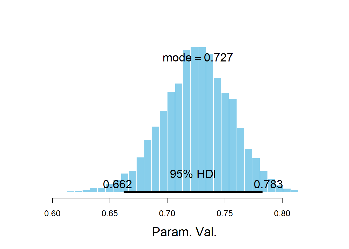

##              ESS   mean median   mode hdiMass hdiLow hdiHigh compVal pGtCompVal
## Param. Val. 2592 0.7253 0.7263 0.7267    0.95 0.6619  0.7829      NA         NA
##             ROPElow ROPEhigh pLtROPE pInROPE pGtROPE
## Param. Val.      NA       NA      NA      NA      NA

Example 19.3 Summarize and describe the posterior distribution of \(\mu\).

\iffalse{} Solution. to Example 19.3

The posterior distribution of \(\mu\) is approximate Normal with a posterior mean of about 0.73 and a posterior standard deviation of 0.03. There is a posterior probability of 95% that the league-wide player average free throw percentage is between 0.67 and 0.79.

Now we’ll compare the posterior means of the individual \(\theta\) parameters to the individual free throw percentages.

# In posterior_sample list, the first two entries correspond to kappa and mu, so we remove them.
player_summary[c("posterior_mean", "posterior_SD")] =
  summary(posterior_sample)$statistics[-(1:2), c("Mean", "SD")]
knitr::kable(player_summary, digits = 3)

player	FTA	FT	FTpct	posterior_mean	posterior_SD
James Nunnally	0	0	NaN	0.726	0.116
Iman Shumpert	0	0	NaN	0.724	0.117
Vince Edwards	0	0	NaN	0.725	0.117
Zhou Qi	0	0	NaN	0.729	0.115
Gary Clark	6	6	1.000	0.801	0.090
Marquese Chriss	7	6	0.857	0.767	0.090
Brandon Knight	11	9	0.818	0.763	0.083
Isaiah Hartenstein	14	11	0.786	0.754	0.079
Carmelo Anthony	22	15	0.682	0.701	0.074
Austin Rivers	26	14	0.538	0.610	0.078
Michael Carter-Williams	26	12	0.462	0.563	0.080
Nene Hilario	31	22	0.710	0.717	0.064
Kenneth Faried	44	24	0.545	0.595	0.065
Gerald Green	49	39	0.796	0.778	0.051
P.J. Tucker	51	33	0.647	0.667	0.057
Danuel House	55	45	0.818	0.798	0.047
James Ennis	58	42	0.724	0.724	0.052
Eric Gordon	118	93	0.788	0.781	0.036
Chris Paul	121	100	0.826	0.815	0.033
Clint Capela	174	109	0.626	0.636	0.035
James Harden	609	529	0.869	0.865	0.014

Example 19.4 Use the table above to answer the following questions.

What is the posterior mean of \(\theta\) for players with no attempts? Why does this make sense?
For which players in the posterior mean closest to the observed free throw percentage? Why?
Examine the player-by-player posterior SDs. Which players have the smallest posterior SDs? Why?

\iffalse{} Solution. to Example 19.4

The posterior mean of \(\theta\) for players with zero attempts is just the posterior mean of \(\mu\), our estimate of the league-wide average.
The posterior mean closest to the observed free throw percentage for players with a greater number of attempts because for these players the data has more influence than the prior.
As a player’s number of attempts increases, there is less uncertainty about the value of \(\theta\) for that player, so the player’s posterior SD decreases.

If each player were analyzed separately, the posterior mean for each player would be close to the sample proportion for that player.

But in the hierarchical model, the posterior mean of each individual \(\theta\) is influenced by \(\mu\) which represents the league-wide average and is affected by the data from all players. So the posterior mean of each player is affected, indirectly, by all the data.

In general, the posterior mean of \(\theta\) for an individual player is a compromise between (1) the observed sample proportion for the player, and (2) the posterior mean of \(\mu\), which represents the league-wide average. As the number of attempts increases, the data (\(\hat{p}_j\)) has more influence on \(\theta_j\) than \(\mu\) does. We say that the individual posterior means of \(\theta\) are “shrunk toward” the overall posterior mean \(\mu\). Players who have the fewest free throw attempts experience the most shrinkage. In some sense, the estimate for a player with few observed attempts “borrows” information from the other players. The idea of shrinkage is similar in a sense to regression to the mean.

players = player_summary[!is.na(player_summary$FTpct), ]
plot(c(1:3, 0:1), type = 'n',
     ylim = range(players[, "FTpct"]),
     ylab = "",
     xlim = c(1, 3), xaxt = 'n')
text(x = rep(2, nrow(players)), y = players[, "posterior_mean"],
     labels = players[, "player"],
     cex = 0.5, adj = 0)
segments(x0 = rep(1, nrow(players)),
         y0 = players[, "FTpct"],
         x1 = rep(2, nrow(players)),
         y1 = players[, "posterior_mean"])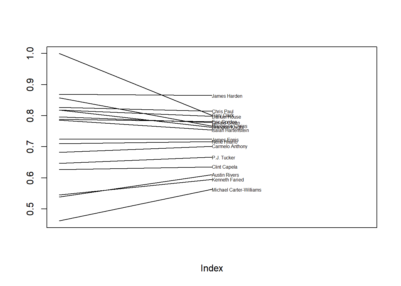

ShinyStan provides a nice interface to interactively investigate the posterior distribution.

library(shinystan)

rockets_sso <- as.shinystan(posterior_sample, model_name = "Houston Rockets Free Throws")
rockets_sso <- drop_parameters(rockets_sso, pars = c("kappa"))
launch_shinystan(rockets_sso)