7.1 Posterior predictive checking

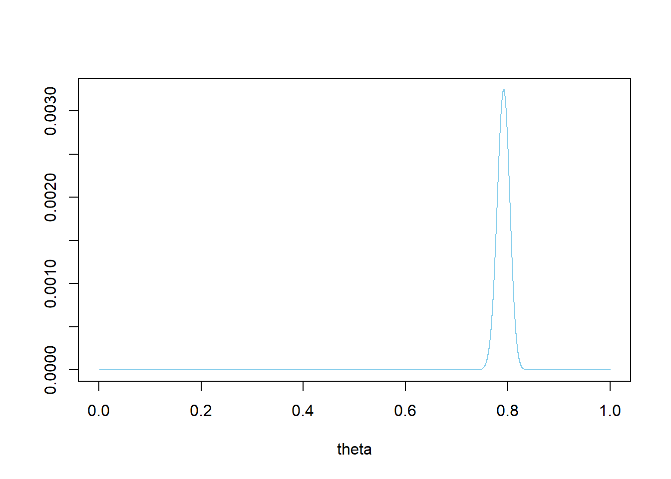
Example 7.3 Continuing the previous example, suppose that before collecting data for our sample of Cal Poly students, we had based our prior distribution off the FiveThirtyEight data. Suppose we assume a prior distribution that is proportional to $\theta^{864}(1-\theta)^{227}$ for $\theta$ values in the grid. (We will see where such a distribution might come from later.)

Plot the prior distribution. What does this say about our prior beliefs?
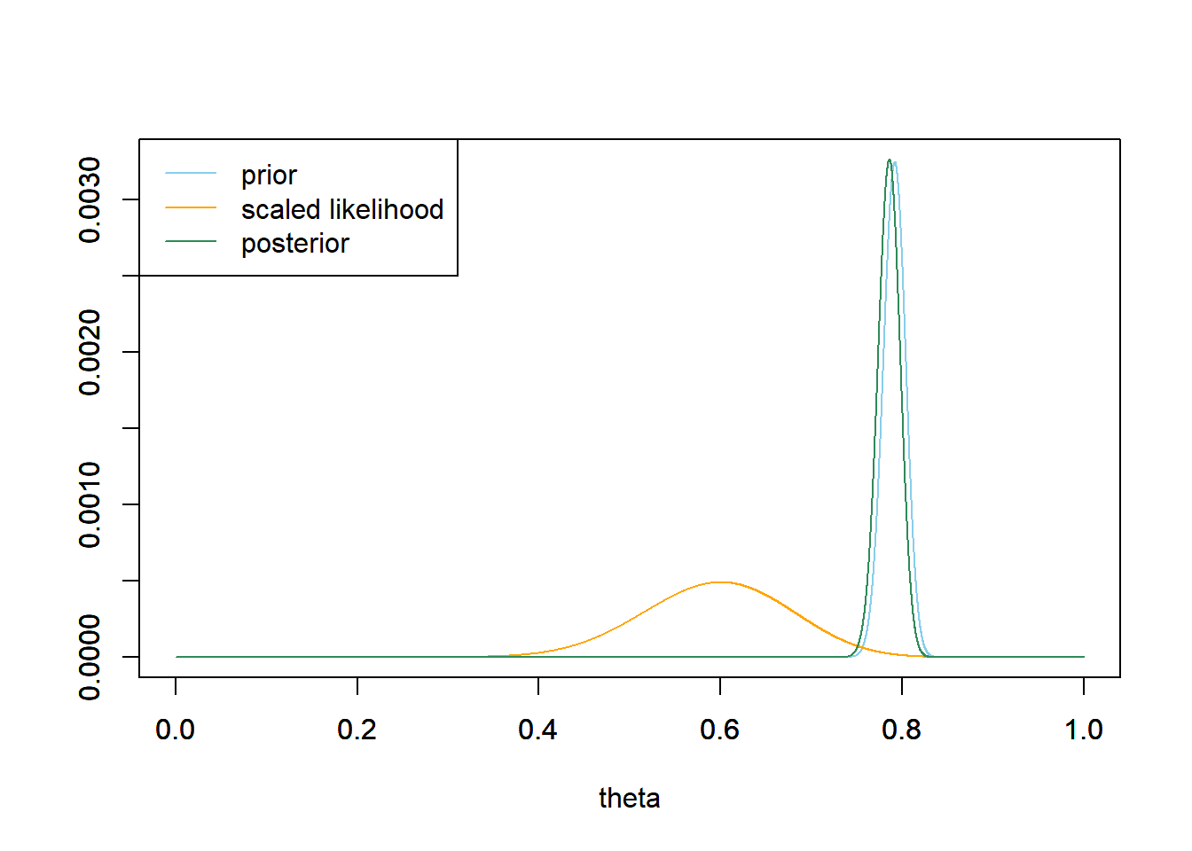
Now suppose we randomly select a sample of 35 Cal Poly students and 21 students prefer data as singular. Plot the prior and likelihood, and find the posterior distribution and plot it. Have our beliefs about $\theta$ changed? Why?
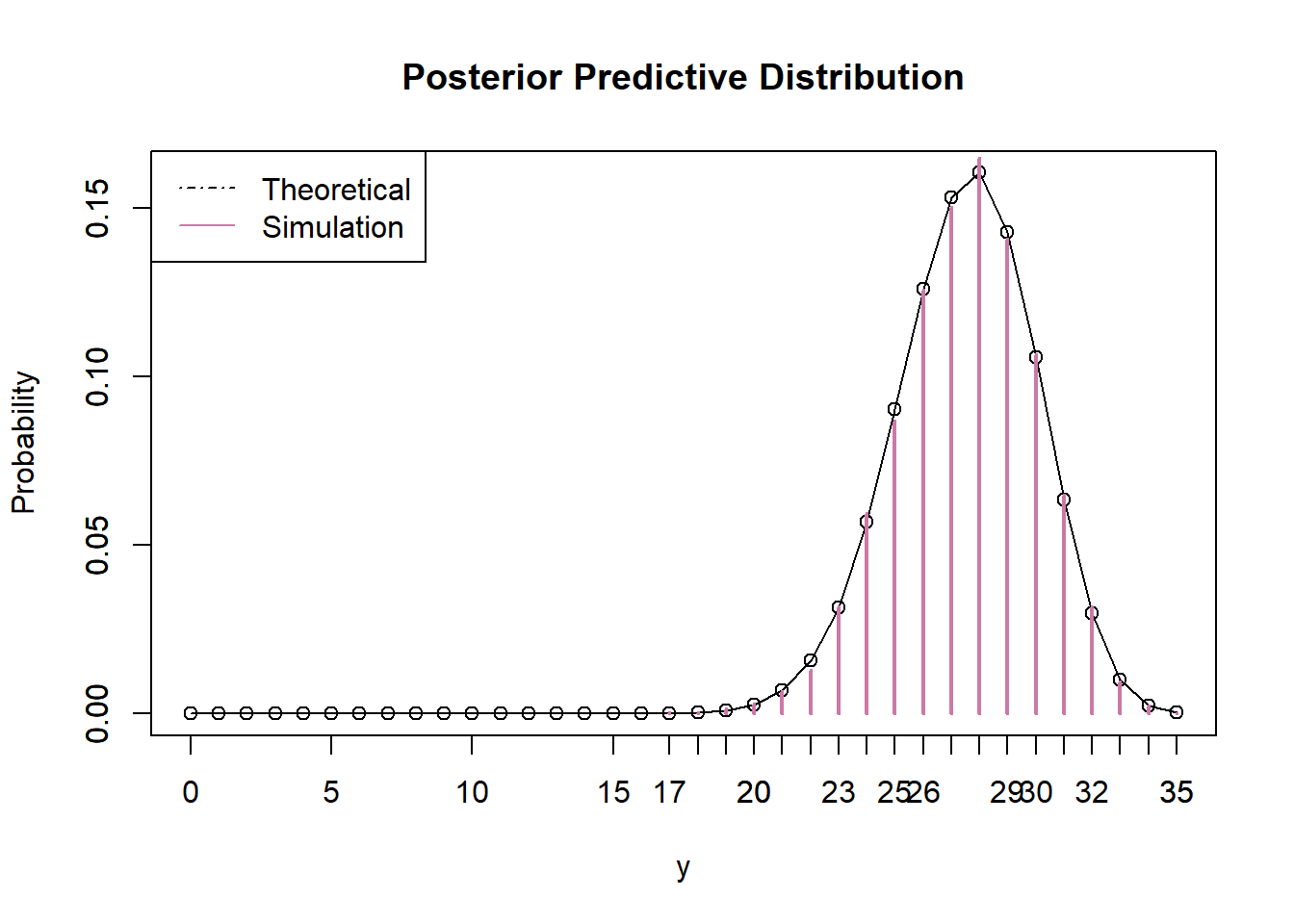
Find the posterior predictive distribution corresponding to samples of size 35. Compare the observed sample value of 21/35 with the posterior predictive distribution. What do you notice? Does this indicate problems with the model?

\iffalse{} Solution. to Example 7.3

We have a very strong prior belief that $\theta$ is close to 0.79; the prior SD is only 0.012. There is a prior probability of 98% that between 76% and 82% of Cal Poly students prefer data as singular.

# prior
theta = seq(0, 1, 0.0001)
prior = theta ^ 864 * (1 - theta) ^ 227
prior = prior / sum(prior)

ylim = c(0, max(prior))
plot(theta, prior, type='l', xlim=c(0, 1), ylim=ylim, col="skyblue", xlab='theta', ylab='')

# prior mean
prior_ev = sum(theta * prior)
prior_ev

## [1] 0.7914

# prior variance
prior_var = sum(theta ^ 2 * prior) - prior_ev ^ 2

# prior sd
sqrt(prior_var)

## [1] 0.01228

# prior 98% credible interval
prior_cdf = cumsum(prior)
c(theta[max(which(prior_cdf <= 0.01))], theta[min(which(prior_cdf >= 0.99))])

## [1] 0.7620 0.8192

Our posterior distribution has barely changed from the prior. Even though the sample proportion is 21/35 = 0.61, our prior beliefs were so strong (represented by the small prior SD) that a sample of size 35 isn’t very convincing.

# data
n = 35 # sample size
y = 21 # sample count of success

# likelihood, using binomial
likelihood = dbinom(y, n, theta) # function of theta

# posterior
product = likelihood * prior
posterior = product / sum(product)

# posterior mean
posterior_ev = sum(theta * posterior)
posterior_ev

## [1] 0.7855

# posterior variance
posterior_var = sum(theta ^ 2 * posterior) - posterior_ev ^ 2

# posterior sd
sqrt(posterior_var)

## [1] 0.01222

# posterior 98% credible interval
posterior_cdf = cumsum(posterior)
c(theta[max(which(posterior_cdf <= 0.01))], theta[min(which(posterior_cdf >= 0.99))])

## [1] 0.7562 0.8131

According to the posterior predictive distribution, it is very unlikely to observe a sample with only 21 students preferring data as singular; only about 1% of examples are this extreme. However, remember that the posterior predictive distribution is based on the observed data. So we’re saying that based on the fact that we observed 21 students in a sample of 35 preferring data as singular it would be unlikely to observe 21 students in a sample of 35 preferring data as singular????? Seems problematic. In this case, the problem is that the prior is way too strict, and it doesn’t give the data enough say.
```
n = 35

# Predictive simulation
theta_sim = sample(theta, n_sim, replace = TRUE, prob = posterior)

y_sim = rbinom(n_sim, n, theta_sim)

# Predictive distribution
y_predict = 0:n

py_predict = rep(NA, length(y_predict))

for (i in 1:length(y_predict)) {
  py_predict[i] = sum(dbinom(y_predict[i], n, theta) * posterior) # posterior
}

    # Prediction interval
sum(py_predict[y_predict <= y])
```
```
## [1] 0.01105
```

A Bayesian model is composed of both a model for the data (likelihood) and a prior distribution on model parameters.

Predictive distributions can be used as tools in model checking. Posterior predictive checking involves comparing the observed data to simulated samples (or some summary statistics) generated from the posterior predictive distribution. We’ll focus on graphical checks: Compare plots for the observed data with those for simulated samples. Systematic differences between simulated samples and observed data indicate potential shortcomings of the model.

If the model fits the data, then replicated data generated under the model should look similar to the observed data. If the observed data is not plausible under the posterior predictive distribution, then this could indicate that the model is not a good fit for the data. (“Based on the data we observed, we conclude that it would be unlikely to observe the data we observed???”)

However, a problematic model isn’t necessarily due to the prior. Remember that a Bayesian model consists of both a prior and a likelihood, so model mis-specification can occur in the prior or likelihood or both. The form of the likelihood is also based on subjective assumptions about the variables being measured and how the data are collected. Posterior predictive checking can help assess whether these assumptions are reasonable in light of the observed data.

Example 7.4 A basketball player will attempt a sequence of 20 free throws. Our model assumes

The probability that the player successfully makes any particular free throw attempt is $\theta$.
A Uniform prior distribution for $\theta$ values in a grid from 0 to 1.
Conditional on $\theta$, the number of successfully made attempts has a Binomial(20, $\theta$) distribution. (This determines the likelihood.)

Suppose the player misses her first 10 attempts and makes her second 10 attempts. Does this data seem consistent with the model?
Explain how you could use posterior predictive checking to check the fit of the model.

\iffalse{} Solution. to Example 7.4

Remember that one condition of a Binomial model is independence of trials: the probability of success on a shot should not depend on the results of previous shots. However, independence seems to be violated here, since the shooter has a long hot streak followed by a long cold streak. So a Binomial model might not be appropriate.
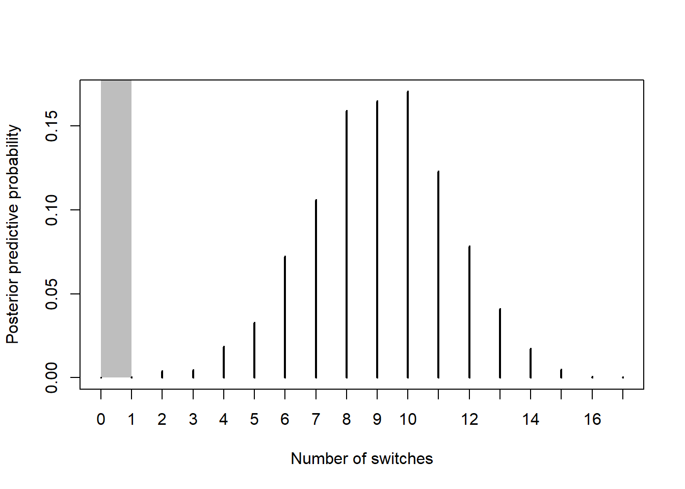
We’re particularly concerned about the independence assumption, so how could we check that? For example, the data seems consistent with a value of $\theta=0.5$, but if the trials were independent, you would expect to see more alterations between makes and misses. So one way to measure degree of dependence is to count the number of “switches” between makes and misses. For the observed data there is only 1 switch. We can use simulation to approximate the posterior predictive distribution of the number of switches assuming the model is true, and then we can see if a value of 1 (the observed number of switches) would be consistent with the model.
1. Find the posterior distribution of $\theta$. Simulate a value of $\theta$ from its posterior distribution.
2. Given $\theta$, simulate a sequence of 20 independent success/failure trials with probability of success $\theta$ on each trial. Compute the number of switches for the sequence. (Since we’re interested in the number of switches, we have to generate the individual success/failure results, and not just the total number of successes).
3. Repeat many times, recording the total number of switches each time. Summarize the values to approximate the posterior predictive distribution of the number of switches.
See the simulation results below. It would be very unlikely to observe only 1 switch in 20 independent trials. Therefore, the proposed model does not fit the observed data well. There is evidence that the assumption of independence is violated.
```
theta = seq(0, 1, 0.0001)

# prior
prior = rep(1, length(theta))
prior = prior / sum(prior)

# data
n = 20 # sample size
y = 10 # sample count of success

# likelihood, using binomial
likelihood = dbinom(y, n, theta) # function of theta

# posterior
product = likelihood * prior
posterior = product / sum(product)

# predictive simulation

n_sim = 10000

switches = rep(NA, n_sim)

for (r in 1:n_sim){
  theta_sim = sample(theta, 1, replace = TRUE, prob = posterior)
  trials_sim = rbinom(n, 1, theta_sim)
  switches[r] = length(rle(trials_sim)$lengths) - 1 # built in function
}

plot(table(switches) / n_sim,
 xlab = "Number of switches",
 ylab = "Posterior predictive probability",
 panel.first = rect(0, 0, 1, 1, col='gray', border=NA))
```
```
sum(switches <= 1) / n_sim
```
```
## [1] 0.0005
```