3.2 Interpretations of probability
In the previous section we encountered a variety of scenarios which involved uncertainty, a.k.a. randomness. Just as there are a few “types” of randomness, there are a few ways of interpreting probability, most notably, long run relative frequency and subjective probability.
3.2.1 Long run relative frequency
One of the oldest documented5 problems in probability is the following: If three fair six-sided dice are rolled, what is more likely: a sum of 9 or a sum of 10? Let’s try to answer this question by simply rolling dice and seeing if a sum of 9 or 10 happens more frequently. Roll three fair six-sided dice, find the sum, repeat many times, and see how often we get a sum of 9 versus a sum of 10. Of course, this would be a time consuming process by hand, but it’s quick and easy on a computer. Figure 3.1 displays the result of one million repetitions of this process, each repetition resulting in the sum of three rolls. A sum of 9 occurred in 115384 repetitions and a sum of 10 occurred in 125005 repetitions. Comparing these frequencies, our results suggest that a sum of 10 is more likely than a sum of 9.
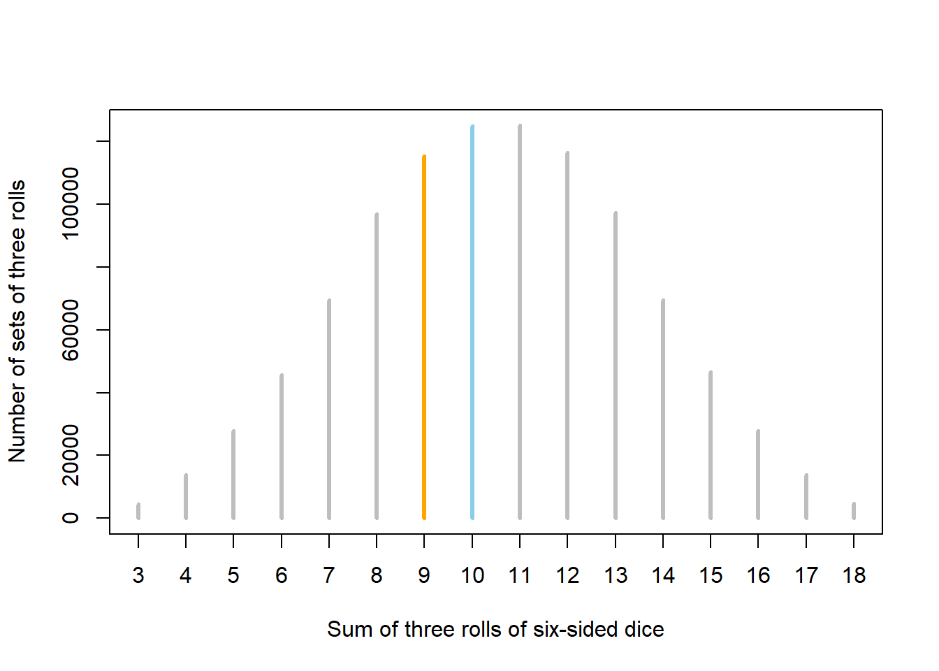
Figure 3.1: Results of one million sets of three rolls of fair six-sided dice. Sets in which the sum of the dice is 9 (10) are represented by orange (blue) spike.
In the previous problem we assessed relative likelihoods by repeating the process many times. This is the idea behind the relative frequency interpretation of probability. We’ll investigate this idea further in the context of what is probably the most iconic random process: coin flipping.
We might all agree that the probability that a single flip of a fair coin lands on heads is 1/2, a.k.a., 0.5, a.k.a, 50%. After all, the notion of “fairness” implies that the two outcomes, heads and tails, should be equally likely, so we have a “50/50 chance” of heads. But how else can we interpret this 50%? As in the dice rolling problem, we can consider what would happen if we flipped the coin main times. Now, if we would flipped the coin twice, we wouldn’t expect to necessarily see one head and one tail. But in many flips, we might expect to see heads on something close to 50% of flips.
Let’s try this out. Table 3.1 displays the results of 10 flips of a fair coin. The first column is the flip number and the second column is the result of the flip. The third column displays the running proportion of flips that result in H. For example, the first flip results in T so the running proportion of H after 1 flip is 0/1; the first two flips result in (T, H) so the running proportion of H after 2 flips is 1/2; and so on. Figure 3.2 plots the running proportion of H by the number of flips. We see that with just a small number of flips, the proportion of H fluctuates considerably and is not guaranteed to be close to 0.5. Of course, the results depend on the particular sequence of coin flips. We encourage you to flip a coin 10 times and compare your results.
| Flip | Result | Running count of H | Running proportion of H |
|---|---|---|---|
| 1 | T | 0 | 0.000 |
| 2 | H | 1 | 0.500 |
| 3 | T | 1 | 0.333 |
| 4 | H | 2 | 0.500 |
| 5 | H | 3 | 0.600 |
| 6 | H | 4 | 0.667 |
| 7 | H | 5 | 0.714 |
| 8 | T | 5 | 0.625 |
| 9 | T | 5 | 0.556 |
| 10 | T | 5 | 0.500 |
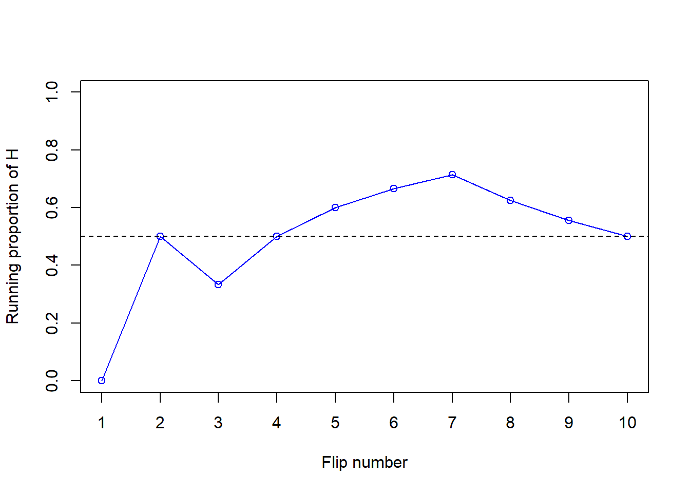
Figure 3.2: Running proportion of H versus number of flips for the 10 coin flips in Table 3.1.
Now we’ll flip the coin 90 more times for a total of 100 flips. The plot on the left in Figure 3.3 summarizes the results, while the plot on the right also displays the results for 3 additional sets of 100 flips. The running proportion fluctuates considerably in the early stages, but settles down and tends to get closer to 0.5 as the number of flips increases. However, each of the fours sets results in a different proportion of heads after 100 flips: 0.5 (blue), 0.44 (orange), 0.56 (green), 0.56 (purple). Even after 100 flips the proportion of flips that result in H isn’t guaranteed to be very close to 0.5.
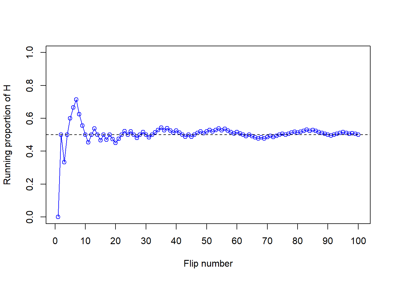
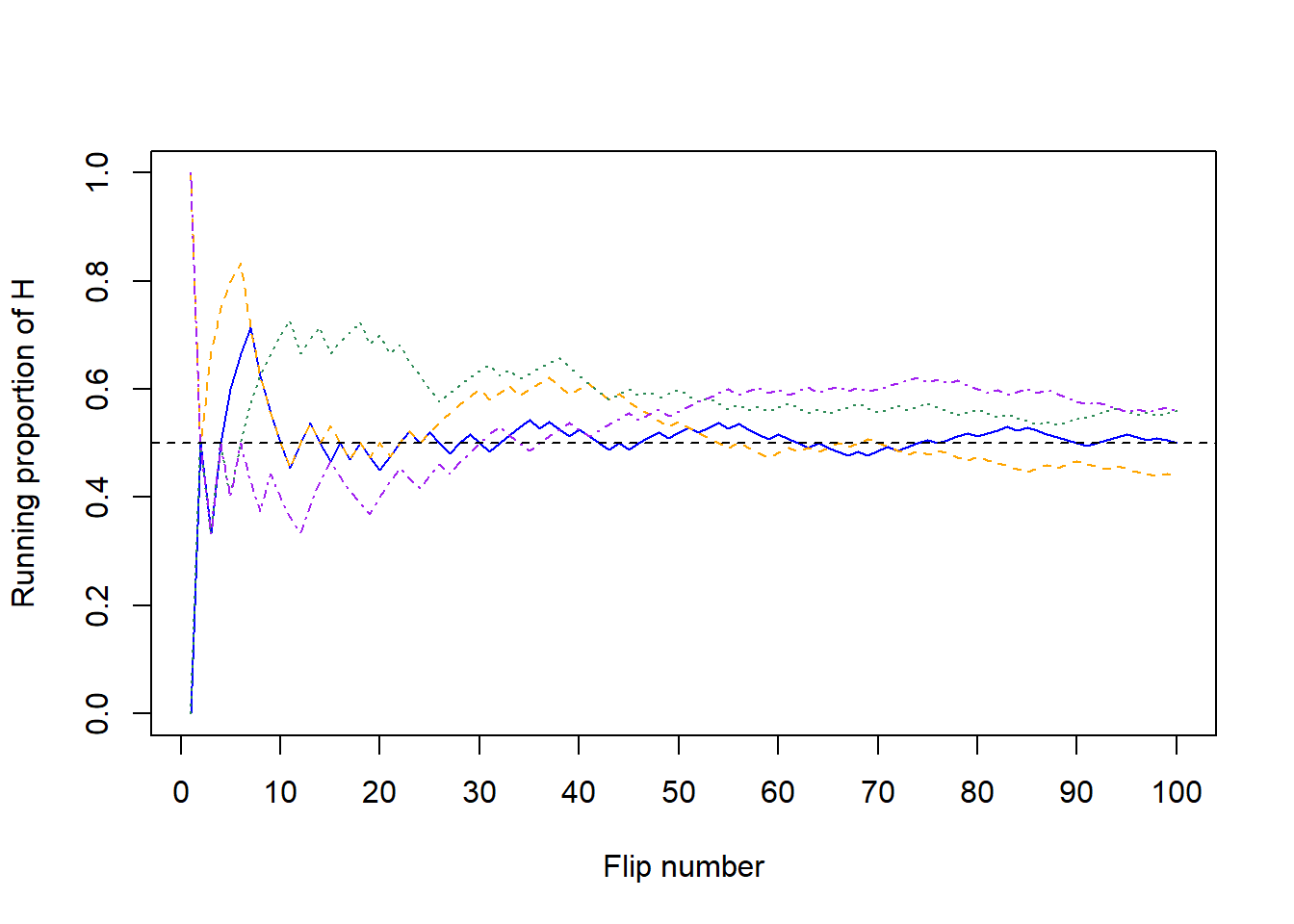
Figure 3.3: Running proportion of H versus number of flips for four sets of 100 coin flips.
Now for each set of 100 flips, we’ll flip the coin 900 more times for a total of 1000 flips in each of the four sets. The plot on the left in Figure 3.4 summarizes the results for our original set, while the plot on the right also displays the results for the three additional sets from Figure 3.4. Again, the running proportion fluctuates considerably in the early stages, but settles down and tends to get closer to 0.5 as the number of flips increases. Compared to the results after 100 flips, there is less variability between sets in the proportion of H after 1000 flips: 0.51 (blue), 0.488 (orange), 0.525 (green), 0.492 (purple). Now, even after 1000 flips the proportion of flips that result in H isn’t guaranteed to be exactly 0.5, but we see a tendency for the proportion to get closer to 0.5 as the number of flips increases.
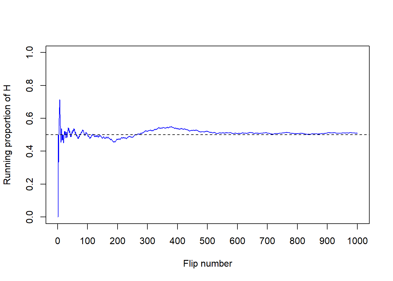
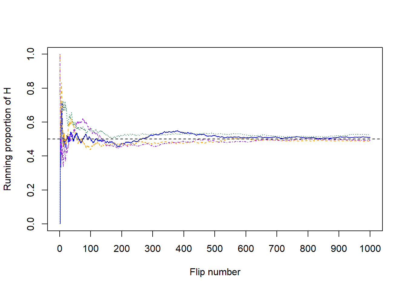
Figure 3.4: Running proportion of H versus number of flips for four sets of 1000 coin flips.
In summary, in a large number of flips of a fair coin we expect about 50% of flips to result in H. That is, the probability that a flip of a fair coin results in H can be interpreted as the long run proportion of flips that result in H, or in other words, the long run relative frequency of H.
In general, the probability of an event associated with a random phenomenon can be interpreted as a long run proportion or long run relative frequency: the probability of the event is the proportion of times that the event would occur in a very large number6 of hypothetical repetitions of the random phenomenon.
The long run relative frequency interpretation of probability can be applied when a situation can be repeated numerous times, at least conceptually, and an outcome can be observed for each repetition. One benefit of the relative frequency interpretation is that the probability of an event can be approximated by simulating the random phenomenon a large number of times and determining the proportion of simulated repetitions on which the event occurred out of the total number of repetitions in the simulation. A simulation involves an artificial recreation of the random phenomenon, usually using a computer. After many repetitions the relative frequency of the event will settle down to a single constant value, and that value is the approximately the probability of the event.
Of course, the accuracy of simulation-based approximations of probabilities depends on how well the simulation represents the actual random phenomenon. Conducting a simulation can involve many assumptions which influence the results. Simulating many flips of a fair coin is one thing; simulating an entire NFL season and the winner of the Superbowl is an entirely different story.
3.2.2 Subjective probability
The long run relative frequency interpretation is natural in repeatable situations like flipping coins, rolling dice, drawing Powerballs, or randomly selecting Cal Poly students.
On the other hand, it is difficult to conceptualize some scenarios in the long run. The next Superbowl will only be played once, the 2024 U.S. Presidential Election will only be conducted once (we hope), and there was only one April 17, 2009 on which you either did or did not eat an apple. But while these situations are not naturally repeatable they still involve randomness (uncertainty) and it is still reasonable to assign probabilities. At this point in time we might think that the Kansas City Chiefs are more likely than the Philadelphia Eagles to win Superbowl 2022 and that President Biden is more likely than Dwayne Johnson to win the U.S. 2024 Presidential Election. If you’ve always been an apple-a-day person, you might think there’s a good chance you ate one on April 17, 2009. It is still reasonable to assign probabilities to quantify such assessments even when an uncertain phenomenon is not repeated.
However, the meaning of probability does seem different in a physically repeatable situations like coin flips than in single occurrences like the 2022 Superbowl. For example, as of Dec 30, 2021,
- According to FiveThirtyEight, the Kansas City Chiefs have a 26% chance of winning the 2022 Superbowl, and the Green Bay Packers have a 24% chance.
- According to Football Outsiders, the Kansas City Chiefs have a 19.4% chance of winning the 2022 Superbowl, and the Green Bay Packers have a 14% chance.
- As reported by CBS Sports, the Kansas City Chiefs have a 20% chance of winning the 2022 Superbowl, and the Green Bay Packers have a 21% chance.
Each source, as well as many others, assigns different probabilities to the Chiefs and Packers winning. Which source, if any, is “correct”?
When the situation involves a fair coin flip, we could perform a simulation to see that the long run proportion of flips that land on H is 0.5, and so the probability that a fair coin flip lands on H is 0.5. Even though the actual 2022 Superbowl will only happen once, we could still perform a simulation involving hypothetical repetitions. However, simulating the Superbowl involves first simulating the 2021-2022 season to determine the playoff matchups, then simulating the playoffs to see which teams make the Superbowl, then simulating the Superbowl matchup itself. And simulating the season involves simulating all the individual games. Even just simulating a single game involves many assumptions; differences in opinions with regards to these assumptions can lead to different probabilities. For example, on Dec 30, according to FiveThirtyEight the Eagles had a 55% chance of beating the Washington Football Team in their game on Jan 2, but according to numberFire it was 65%. (Let’s hope the Eagles won.) Even though the differences in probabilities between sources are often small, many small differences over the course of the season could result in large differences in predictions for the Superbowl champion.
Unlike physically repeatable situations such as flipping a coin, there is no single set of “rules” for conducting a simulation of a season of football games or the Superbowl champion. Therefore, there is no single long run relative frequency that determines the probability. Instead we consider subjective probability.
A subjective (a.k.a. personal) probability describes the degree of likelihood a given individual assigns to a certain event. As the name suggests, different individuals (or probabilistic models) might have different subjective probabilities for the same event. In contrast, in the long run relative frequency interpretation the probability is agreed to be defined as the long run relative frequency, a single number.
Think of subjective probabilities as measuring relative degrees of likelihood, uncertainty, or plausibility rather than long run relative frequencies. For example, in the FiveThirtyEight forecast (as of Dec 30), the Chiefs (26% chance) are about 3.25 times more likely to win the 2022 Superbowl than the Cowboys (8% chance); \(3.25 = 26 / 8\). Relative likelihoods can also be compared across different forecasts or scenarios. For example, FiveThirtyEight believes that the Packers are about 1.7 times more likely to win the Superbowl than Football Outsiders does (24% versus 14%). Also, FiveThirtyEight believes that the likelihood that a fair coin lands on H is about 1.92 times larger than the likelihood that the Chiefs win the 2022 Superbowl.
The FiveThirtyEight NFL predictions are the output of a probabilistic forecast. A probabilistic forecast combines observed data and statistical models to make predictions. Rather than providing a single prediction (such as “the Chiefs will win the 2022 Superbowl”), probabilistic forecasts provide a range of scenarios and their relative likelihoods. Such forecasts are subjective in nature, relying upon the data used and assumptions of the model. Changing the data or assumptions can result in different forecasts and probabilities. In particular, probabilistic forecasts are usually revised over time as more data becomes available.
Simulations can also be based on subjective probabilities. If we were to conduct a simulation consistent with FiveThirtyEight’s model (as of Dec 30), then in about 26% of repetitions the Chiefs would win the Superbowl, and in about 8% of repetitions the Cowboys would win. Of course, different sets of subjective probabilities correspond to different assumptions and different ways of conducting the simulation.
Subjective probabilities can be calibrated by weighing the relative favorability of different bets, as in the following example.
Example 3.2 What is your subjective probability that Professor Ross has a TikTok account? Consider the following two bets, and suppse you must choose only one7.
- You win $100 if Professor Ross has a TikTok account, and you win nothing otherwise.
- A box contains 40 green and 60 gold marbles that are otherwise identical. The marbles are thoroughly mixed and one marble is selected at random. You win $100 if the selected marble is green, and you win nothing otherwise.
- Which of the above bets would you prefer? Or are you completely indifferent? What does this say about your subjective probability that Professor Ross has a Tik Tok account?
- If you preferred bet B to bet A, consider bet C which has a similar setup to B but now there are 20 green and 80 gold marbles. Do you prefer bet A or bet C? What does this say about your subjective probability that Professor Ross has a Tik Tok account?
- If you preferred bet A to bet B, consider bet D which has a similar setup to B but now there are 60 green and 40 gold marbles. Do you prefer bet A or bet D? What does this say about your subjective probability that Professor Ross has a Tik Tok account?
- Continue to consider different numbers of green and gold marbles. Can you zero in on your subjective probability?
\iffalse{} Solution. to Example 3.2
Show/hide solution
- Since the two bets have the same payouts, you should prefer the one that gives you a greater chance of winning! If you choose bet B you have a 40% chance of winning.
- If you prefer bet B to bet A, then your subjective probability that Professor Ross has a TikTok account is less than 40%.
- If you prefer bet A to bet B, then your subjective probability that Professor Ross has a TikTok account is greater than 40%.
- If you’re indifferent between bets A and B, then your subjective probability that Professor Ross has a TikTok account is equal to 40%.
- If you choose bet C you have a 20% chance of winning.
- If you prefer bet C to bet A, then your subjective probability that Professor Ross has a TikTok account is less than 20%.
- If you prefer bet A to bet C, then your subjective probability that Professor Ross has a TikTok account is greater than 20%.
- If you’re indifferent between bets A and C, then your subjective probability that Professor Ross has a TikTok account is equal to 20%.
- If you choose bet D you have a 60% chance of winning.
- If you prefer bet D to bet A, then your subjective probability that Professor Ross has a TikTok account is less than 60%.
- If you prefer bet A to bet D, then your subjective probability that Professor Ross has a TikTok account is greater than 60%.
- If you’re indifferent between bets A and D, then your subjective probability that Professor Ross has a TikTok account is equal to 60%.
- Continuing in this way you can narrow down your subjective probability. For example, if you prefer bet B to bet A and bet A to bet C, your subjective probability is between 20% and 40%. Then you might consider bet E corresponding to 30 gold marbles and 70 green to determine if you subjective probability is greater than or less than 30%. At some point it will be hard to choose, and you will be in the ballpark of your subjective probability. (Think of it like going to the eye doctor: “which is better: 1 or 2?” At some point you can’t really see a difference.)
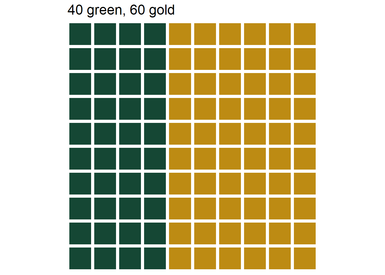
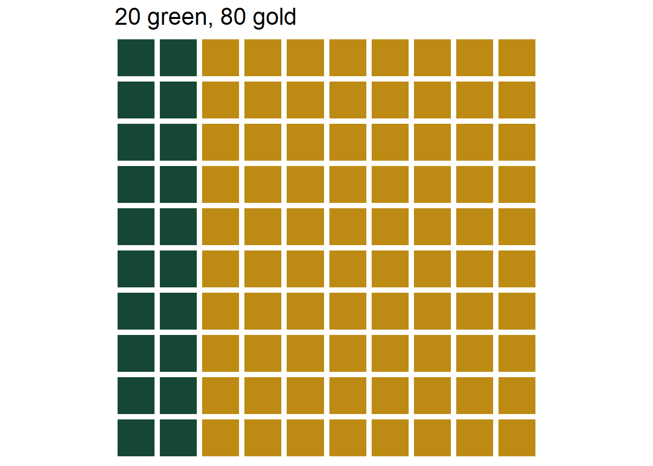
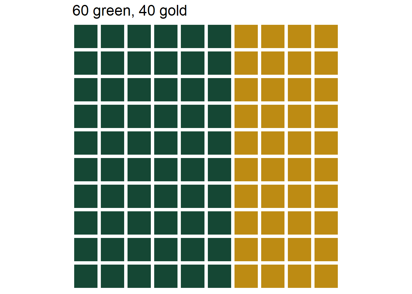
Figure 3.5: The three marble bins in Example 3.2. Left: Bet A, 40% chance of selecting green. Middle: Bet B, 20% chance of selecting green. Left: Bet C, 60% chance of selecting green.
Of course, the strategy in the above example isn’t an exact science, and there is a lot of behavioral psychology behind how people make choices in situations like this, especially when betting with real money. But the example provides a very rough idea of how you might discern a subjective probability of an event. The example also illustrates that probabilities can be “personal”; your information or assumptions will influence your assessment of the likelihood.
We close this section with some brief comments about subjectivity. Subjectivity is not bad; “subjective” is not a “dirty” word. Any probability model involves some subjectivity, even when probabilities can be interpreted naturally as long run relative frequencies. For example, assuming a die is fair does not codify an objective truth about the die. Instead, “fairness” reflects a reasonable and tractable mathematical model. In the real world, any “fair” six-sided die has small physical imperfections that cause the six faces to have different probabilities. However, the differences are usually small enough to be ignored for most practical purposes. Assuming that the probability that the die lands on each side is 1/6 is much more tractable than assuming the probability of a 1 is 0.1666666668, the probability of a 2 is 0.1666666665, etc. (Furthermore, measuring the probability of each side so precisely would be extremely difficult.) But assuming that the probability that the die lands on each side is 1/6 is also subjective. We might readily agree to assume that the probability that a six-sided die lands on 1 is 1/6, but we might not reach a concensus on the probability that the Chiefs win the Superbowl. But the fact that there cam be many reasonable probability models for a situation like the 2022 Superbowl does not make the corresponding subjective probabilities any less valid than long run relative frequencies.