Chapter 10 Introduction to Posterior Simulation and JAGS

In the Beta-Binomial model there is a simple expression for the posterior distribution. However, in most problems it is not possible to find the posterior distribution analytically, and therefore we must approximate it.

Example 10.1 Consider Example 8.5 again, in which we wanted to estimate the proportion of Cal Poly students that are left-handed. In that example we specifed a prior by first specifying a prior mean of 0.15 and a prior SD of 0.08 and then we found the corresponding Beta prior. However, when dealing with means and SDs, it is natural — but by no means necessary — to work with Normal distributions. Suppose we want to assume a Normal distribution prior for \(\theta\) with mean 0.15 and SD 0.08. Also suppose that in a sample of 25 Cal Poly students 5 are left-handed. We want to find the posterior distribution.

Note: the Normal distribution prior assigns positive (but small) density outside of (0, 1). So we can either truncate the prior to 0 outside of (0, 1) or just rely on the fact that the likelihood will be 0 for \(\theta\) outside of (0, 1) to assign 0 posterior density outside (0, 1).

Write an expression for the shape of the posterior density. Is this a recognizable probability distribution?
We have seen one method for approximating a posterior distribution. How could you employ it here?

\iffalse{} Solution. to Example 10.1

As always, the posterior density is proportional to the product of the prior density and the likelihood function. \[\begin{align*} \text{Prior:} & & \pi(\theta) & \propto \frac{1}{0.08}\exp\left(-\frac{\left(\theta - 0.15\right)^2}{2(0.08^2)}\right)\\ \text{Likelihood:} & & f(y|\theta) & \propto \theta^5(1-\theta)^{20}\\ \text{Posterior:} & & \pi(\theta | y) & \propto \left(\theta^5(1-\theta)^{20}\right)\left(\frac{1}{0.08}\exp\left(-\frac{\left(\theta - 0.15\right)^2}{2(0.08^2)}\right)\right) \end{align*}\] This is not a recognizable probability density.
We can use grid approximation and treat the continuous parameter \(\theta\) as discrete.

theta = seq(0, 1, 0.0001)

# prior
prior = dnorm(theta, 0.15, 0.08)
prior = prior / sum(prior)

# data
n = 25 # sample size
y = 5 # sample count of success

# likelihood, using binomial
likelihood = dbinom(y, n, theta) # function of theta

# posterior
product = likelihood * prior
posterior = product / sum(product)

# plot
ylim = c(0, max(c(prior, posterior, likelihood / sum(likelihood))))
plot(theta, prior, type='l', xlim=c(0, 1), ylim=ylim, col="skyblue", xlab='theta', ylab='')
par(new=T) 
plot(theta, likelihood / sum(likelihood), type='l', xlim=c(0, 1), ylim=ylim, col="orange", xlab='', ylab='')
par(new=T)
plot(theta, posterior, type='l', xlim=c(0, 1), ylim=ylim, col="seagreen", xlab='', ylab='')
legend("topright", c("prior", "scaled likelihood", "posterior"), lty=1, col=c("skyblue", "orange", "seagreen"))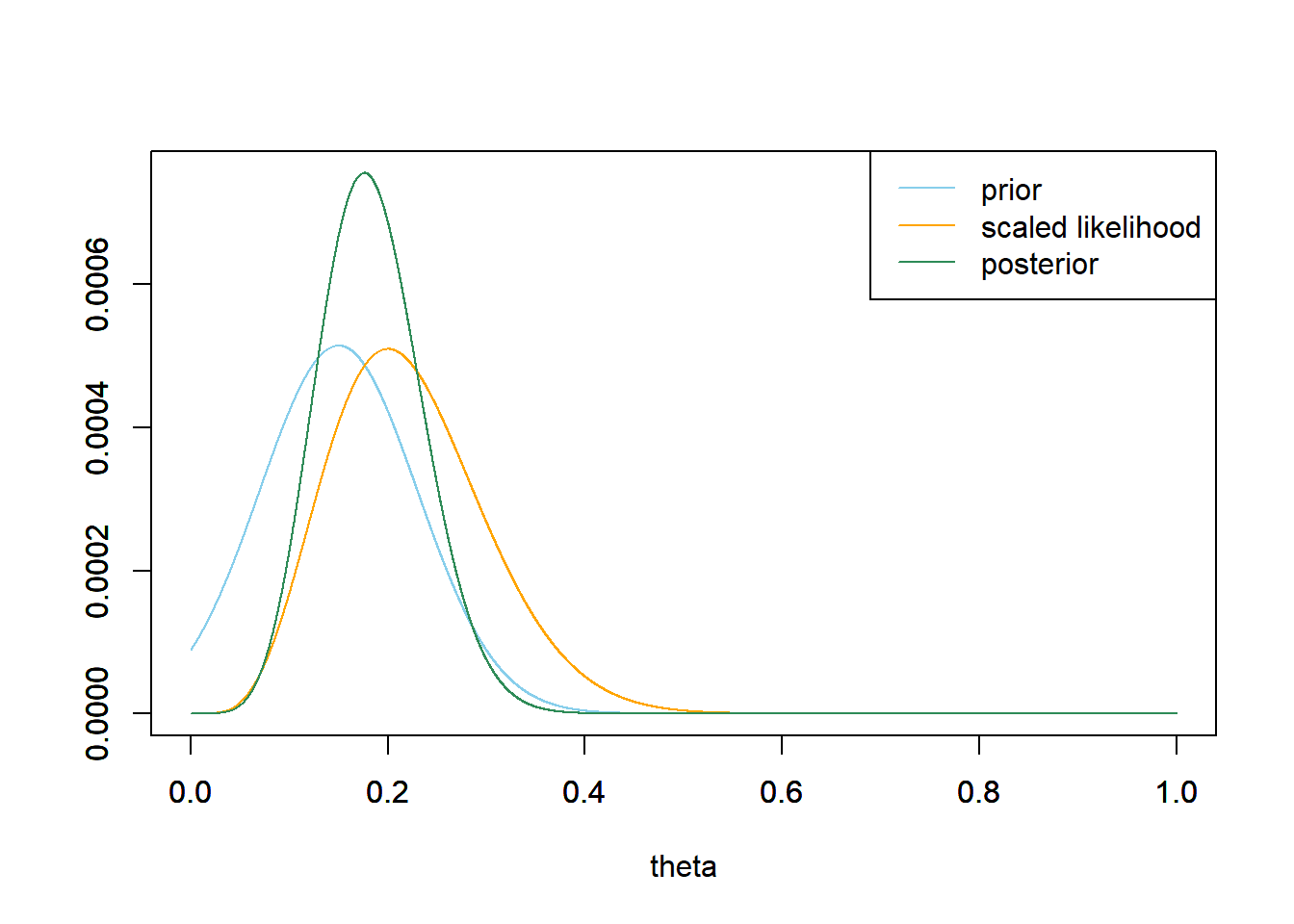

Grid approximation is one method for approximating a posterior distribution. However, finding a sufficiently fine grid approximation suffers from the “curse of dimensionality” and does not work well in multi-parameter problems. For example, suppose you use a grid of 1000 points to approximate the distribution of any single parameter. Then you would need a grid of \(1000^2\) points to approximate the joint distribution of any two parameters, \(1000^3\) points for three parameters, and so on. The size of the grid increases exponentially with the number of parameters and becomes computationally infeasible in problems with more than a few parameters. (And later we’ll see some examples that include hundreds of parameters.) Furthermore, if the posterior density changes very quickly over certain regions, then even finer grids might be needed to provide reliable approximations of the posterior in these regions. (Though if the posterior density is relative smooth over some regions, then we might be able to get away with a coarser grid in these regions.)

The most common way to approximate a posterior distribution is via simulation. The inputs to the simulation are

Observed data \(y\)
Model for the data, \(f(y|\theta)\) which depends on parameters \(\theta\). (This model determines the likelihood function.)
Prior distribution for parameters \(\pi(\theta)\)

We then employ some simulation algorithm to approximate the posterior distribution of \(\theta\) given the observed data \(y\), \(\pi(\theta|y)\), without computing the posterior distribution.

Careful: we have already used simulation to approximate predictive distributions. Here we are primarily focusing on using simulation to approximate the posterior distribution of parameters.

Let’s consider a discrete example first.

Example 10.2 Continuing the kissing study in Example 5.2 where \(\theta\) can only take values 0.1, 0.3, 0.5, 0.7, 0.9. Consider a prior distribution which places probability 1/9, 2/9, 3/9, 2/9, 1/9 on the values 0.1, 0.3, 0.5, 0.7, 0.9, respectively. Suppose that \(y=8\) couples in a sample of size \(n=12\) lean right.

Describe in detail how you could use simulation to approximate the posterior distribution of \(\theta\), without first computing the posterior distribution.
Code and run the simulation. Compare the simulation-based approximation to the true posterior distribution from Example 5.2.
How would the simulation/code change if \(\theta\) had a Beta prior distribution, say Beta(3, 3)?
Suppose that \(n = 1200\) and \(y = 800\). What would be the problem with running the above simulation in this situation? Hint: compute the probability that \(Y\) equals 800 for a Binomial distribution with parameters 1200 and 0.667.

\iffalse{} Solution. to Example 10.2

Remember that the posterior distribution is the conditional distribution of parameters \(\theta\) given the observed data \(y\). Therefore, we need to approximate the conditional distribution of \(\theta\) given \(y=8\) successes in a sample of size \(n=12\).
- Simulate a value of \(\theta\) from the prior distribution.
- Given \(\theta\), simulate a value of \(Y\) from the Binomial distribution with parameters \(n=12\) and \(\theta\).
- Repeat the above steps many times, generating many \((\theta, Y)\) pairs.
- To condition on \(y=8\), discard any \((\theta, Y)\) pairs for which \(Y\) is not 8. Summarize the \(\theta\) values for the remaining pairs to approximate the posterior distribution of \(\theta\). For example, to approximate the posterior probability that \(\theta\) equals 0.7, count the number of repetitions in which \(\theta\) equals 0.7 and \(Y\) equals 8 and divide by the count of repetitions in which \(Y\) equals 8.

See code below. The simulation approximates the posterior distribution fairly well in this case. Notice that we simulate 100,000 \((\theta, Y)\) pairs, but only around 10,000 or so yield a value of \(Y\) equal to 8. Therefore, the posterior approximation is based on roughly 10,000 values, not 100,000.

n_sim = 100000

theta_prior_sim = sample(c(0.1, 0.3, 0.5, 0.7, 0.9), 
                     size = n_sim,
                     replace = TRUE,
                     prob = c(1, 2, 3, 2, 1) / 9)

y_sim = rbinom(n_sim, 12, theta_prior_sim)

kable(head(data.frame(theta_prior_sim, y_sim), 20))

theta_prior_sim	y_sim
0.1	0
0.5	2
0.5	5
0.7	10
0.1	2
0.5	6
0.5	8
0.1	1
0.7	7
0.5	7
0.7	10
0.3	3
0.5	5
0.5	7
0.9	11
0.7	12
0.3	6
0.5	8
0.3	5
0.9	10

theta_post_sim = theta_prior_sim[y_sim == 8]

table(theta_post_sim)

## theta_post_sim
##  0.3  0.5  0.7  0.9 
##  177 4070 5031  253

plot(table(theta_post_sim) / length(theta_post_sim),
 xlab = "theta",
 ylab = "Relative frequency")

# true posterior for comparison
par(new = T)
plot(c(0.3, 0.5, 0.7, 0.9), c(0.0181, 0.4207, 0.5365, 0.0247),
 col = "orange", type = "o",
 xaxt = 'n', yaxt = 'n', xlab = "", ylab = "")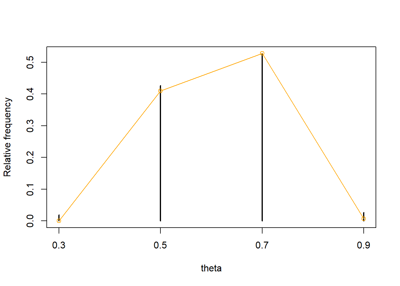

The only difference is that we would first simulate a value of \(\theta\) from its Beta(3, 3) prior distribution (using rbeta). Now any value between 0 and 1 is a possible value of \(\theta\). But we would still approximate the posterior distribution by discarding any \((\theta, Y)\) pairs for which \(Y\) is not equal to 8. Since \(\theta\) is continuous, we could summarize the simulated values with a histogram or density plot.

n_sim = 100000

theta_prior_sim = rbeta(n_sim, 3, 3)

y_sim = rbinom(n_sim, 12, theta_prior_sim)

kable(head(data.frame(theta_prior_sim, y_sim), 20))

theta_prior_sim	y_sim
0.4965	6
0.3985	6
0.4446	6
0.4233	7
0.4427	5
0.5821	6
0.1518	4
0.6136	6
0.7128	6
0.3245	5
0.7393	8
0.3007	4
0.9726	12
0.3001	3
0.2044	1
0.3401	2
0.6289	6
0.7696	11
0.7605	10
0.3823	4

theta_post_sim = theta_prior_sim[y_sim == 8]

hist(theta_post_sim, freq = FALSE,
 xlab = "theta",
 ylab = "Density")
lines(density(theta_post_sim))

# true posterior for comparison
lines(density(rbeta(100000, 3 + 8, 3 + 4)), col = "orange")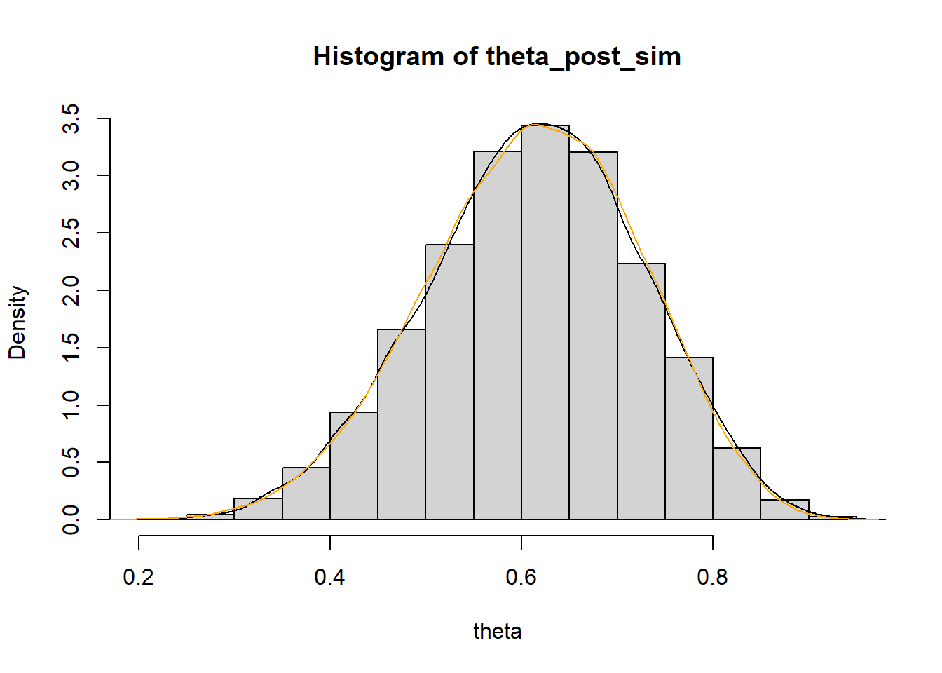

Now we need to approximate the conditional distribution of \(\theta\) given 800 successes in a sample of size \(n=1200\). The probability that \(Y\) equals 800 for a Binomial distribution with parameters 1200 and 2/3 is about 0.024 (dbinom(800, 1200, 2 / 3)). Since the sample proportion 800/1200 = 2/3 maximizes the likelihood of \(y=800\), the probability is even smaller for the other values of \(\theta\).
Therefore, if we generate 100,000 (\(\theta, Y\)) pairs, only a few hundred or so of them would yield \(y=800\) and so the posterior approximation would be unreliable. If we wanted the posterior approximation to be based on 10,000 simulated values from the conditional distribution of \(\theta\) given \(y=8\), we would first have to general about 10 million \((\theta, Y)\) pairs.

In principle, the posterior distribution \(\pi(\theta|y)\) given observed data \(y\) can be found by

simulating many \(\theta\) values from the prior distribution
simulating, for each simulated value of \(\theta\), a \(Y\) value from the corresponding conditional distribution of \(Y\) given \(\theta\) (\(Y\) could be a sample or the value of a sample statistic)
discarding \((\theta, Y)\) pairs for which the simulated \(Y\) value is not equal to the observed \(y\) value
Summarizing the simulated \(\theta\) values for the remaining pairs with \(Y=y\).

However, this is a very computationally inefficient way of approximating the posterior distribution. Unless the sample size is really small, the simulated sample statistic \(Y\) will only match the observed \(y\) value in relatively few samples, simply because in large samples there are just many more possibilities. For example, in 1000 flips of a fair coin, the most likely value of the number of heads is 500, but the probability of exactly 500 heads in 1000 flips is only 0.025. When there are many possibilities, the probability gets stretched fairly thin. Therefore, if we want say 10000 simulated values of \(\theta\) given \(y\), we would have first simulate many, many more values.

The situation is even more extreme when the data is continuous, where the probably of replicating the observed sample is essentially 0.

Therefore, we need more efficient simulation algorithms for approximating posterior distributions. Markov chain Monte Carlo (MCMC) methods¹⁸ provide powerful and widely applicable algorithms for simulating from probability distributions, including complex and high-dimensional distributions. These algorithms include Metropolis-Hastings, Gibbs sampling, Hamiltonian Monte Carlo, among others. We will see later some of the ideas behind MCMC algorithms. However, we will rely on software to carry out MCMC simulations.

theta_prior_sim	y_sim
0.1	0
0.5	2
0.5	5
0.7	10
0.1	2
0.5	6
0.5	8
0.1	1
0.7	7
0.5	7
0.7	10
0.3	3
0.5	5
0.5	7
0.9	11
0.7	12
0.3	6
0.5	8
0.3	5
0.9	10

theta_prior_sim	y_sim
0.1	0
0.5	2
0.5	5
0.7	10
0.1	2
0.5	6
0.5	8
0.1	1
0.7	7
0.5	7
0.7	10
0.3	3
0.5	5
0.5	7
0.9	11
0.7	12
0.3	6
0.5	8
0.3	5
0.9	10

theta_prior_sim	y_sim
0.1	0
0.5	2
0.5	5
0.7	10
0.1	2
0.5	6
0.5	8
0.1	1
0.7	7
0.5	7
0.7	10
0.3	3
0.5	5
0.5	7
0.9	11
0.7	12
0.3	6
0.5	8
0.3	5
0.9	10