10.1 Introduction to JAGS
JAGS19 (“Just Another Gibbs Sampler”) is a stand alone program for performing MCMC simulations. JAGS takes as input a Bayesian model description — prior plus likelihood — and data and returns an MCMC sample from the posterior distribution. JAGS uses a combination of Metropolis sampling, Gibbs sampling, and other MCMC algorithms.
A few JAGS resources:
- JAGS User Manual
- JAGS documentation
- Some notes about JAGS error messages
- Doing Bayesian Data Analysis textbook website
The basic steps of a JAGS program are:
- Load the data
- Define the model: likelihood and prior
- Compile the model in JAGS
- Simulate values from the posterior distribution
- Summarize simulated values and check diagnostics
This section introduces a brief introduction to JAGS in some relatively simple situations.
Using the rjags package, one can interact with JAGS entirely within R.
library(rjags)10.1.1 Load the data
We’ll use the “data is singular” context as an example. Compare the results of JAGS simulations to the results in Chapter 7.
The data could be loaded from a file, or specified via sufficient summary statistics. Here we’ll just load the summary statistics and in later examples we’ll show how to load individual values.
n = 35 # sample size
y = 31 # number of successes
10.1.2 Specify the model: likelihood and prior
A JAGS model specification starts with model. The model provides a textual description of likelihood and prior. This text string will then be passed to JAGS for translation.
Recall that for the Beta-Binomial model, the prior distribution is \(\theta\sim\) Beta\((\alpha, \beta)\) and the likelihood for the total number of successes \(Y\) in a sample of size \(n\) corresponds to \((Y|\theta)\sim\) Binomial\((n, \theta)\). Notice how the following text reflects the model (prior & likelihood).
Note: JAGS syntax is similar to, but not the same, as R syntax. For example, compare dbinom(y, n, theta) in R versus y ~ dbinom(theta, n) in JAGS. See the JAGS user manual for more details. You can use comments with # in JAGS models, similar to R.
model_string <- "model{

  # Likelihood
  y ~ dbinom(theta, n)

  # Prior
  theta ~ dbeta(alpha, beta)
  alpha <- 3 # prior successes
  beta <- 1 # prior failures

}"
Again, the above is just a text string, which we’ll pass to JAGS for translation.
10.1.3 Compile in JAGS
We pass the model (which is just a text string) and the data to JAGS to be compiled via jags.model. The model is defined by the text string via the textConnection function. The model can also be saved in a separate file, with the file name being passed to JAGS. The data is passed to JAGS in a list. In dataList below y = y, n = n maps the data defined by y=31, n=35 to the terms y, n specified in the model_string.
dataList = list(y = y, n = n)

model <- jags.model(file = textConnection(model_string),
                    data = dataList)
## Compiling model graph
## Resolving undeclared variables
## Allocating nodes
## Graph information:
## Observed stochastic nodes: 1
## Unobserved stochastic nodes: 1
## Total graph size: 5
##
## Initializing model10.1.4 Simulate values from the posterior distribution
Simulating values in JAGS is completed in essentially two steps. The update command runs the simulation for a “burn-in” period. The update function merely “warms-up” the simulation, and the values sampled during the update phase are not recorded. (We will discuss “burn-in” in more detail later.)
update(model, n.iter = 1000)After the update phase, we simulate values from the posterior distribution that we’ll actually keep using coda.samples. Using coda.samples arranges the output in a format conducive to using coda, a package which contains helpful functions for summarizing and diagnosing MCMC simulations. The variables to record simulated values for are specified with the variable.names argument. Here there is only a single parameter theta, but we’ll see multi-parameter examples later.
Nrep = 10000 # number of values to simulate

posterior_sample <- coda.samples(model,
                       variable.names = c("theta"),
                       n.iter = Nrep)
10.1.5 Summarizing simulated values and diagnostic checking
Standard R functions like summary and plot can be used to summarize results from coda.samples. We can summarize the simulated values of theta to approximate the posterior distribution.
summary(posterior_sample)##
## Iterations = 2001:12000
## Thinning interval = 1
## Number of chains = 1
## Sample size per chain = 10000
##
## 1. Empirical mean and standard deviation for each variable,
## plus standard error of the mean:
##
## Mean SD Naive SE Time-series SE
## 0.871640 0.053934 0.000539 0.000739
##
## 2. Quantiles for each variable:
##
## 2.5% 25% 50% 75% 97.5%
## 0.746 0.840 0.879 0.911 0.956plot(posterior_sample)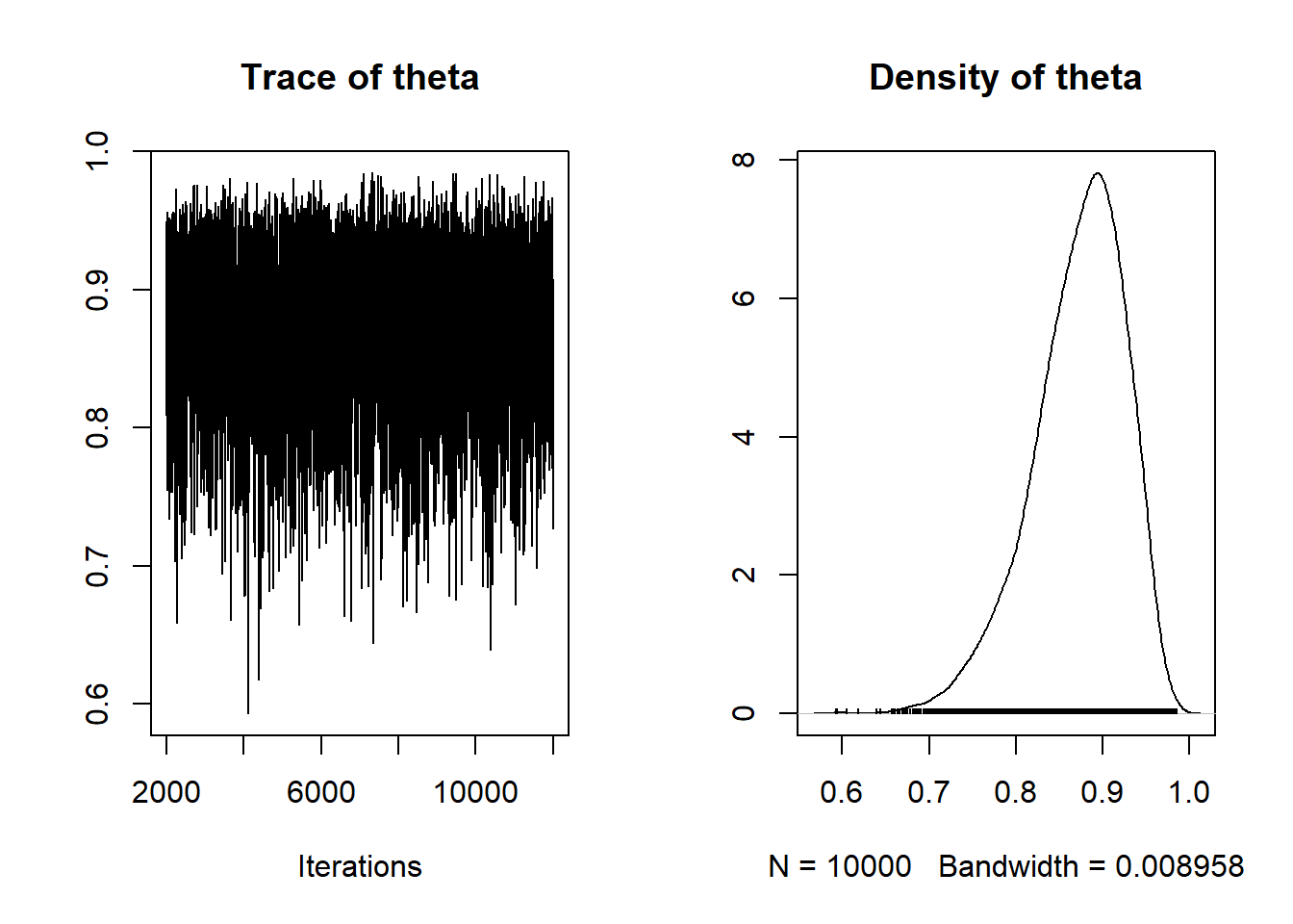
The Doing Bayesian Data Analysis (DBDA2E) textbook package also has some nice functions built in, in particular in the DBD2AE-utilities.R file.
For example, the plotPost functions creates an annotated plot of the posterior distribution along with some summary statistics. (See the DBDA2E documentation for additional arguments.)
source("DBDA2E-utilities.R")##
## *********************************************************************
## Kruschke, J. K. (2015). Doing Bayesian Data Analysis, Second Edition:
## A Tutorial with R, JAGS, and Stan. Academic Press / Elsevier.
## *********************************************************************plotPost(posterior_sample)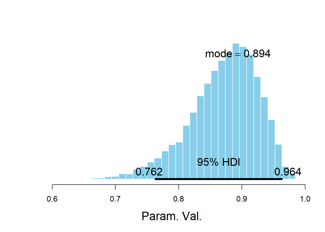
##              ESS   mean median   mode hdiMass hdiLow hdiHigh compVal pGtCompVal
## Param. Val. 5328 0.8716 0.8788 0.8937    0.95 0.7622  0.9642      NA         NA
##             ROPElow ROPEhigh pLtROPE pInROPE pGtROPE
## Param. Val.      NA       NA      NA      NA      NA
The bayesplot R package also provides lots of nice plotting functionality.
library(bayesplot)
mcmc_hist(posterior_sample)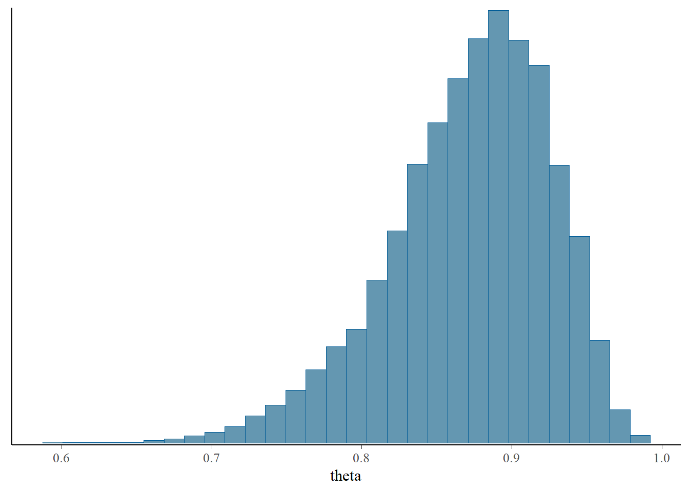
mcmc_dens(posterior_sample)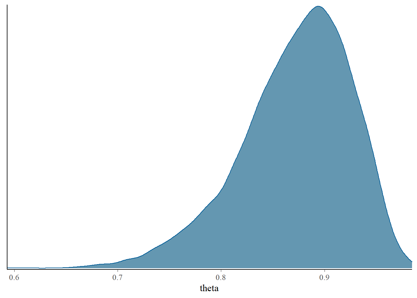
mcmc_trace(posterior_sample)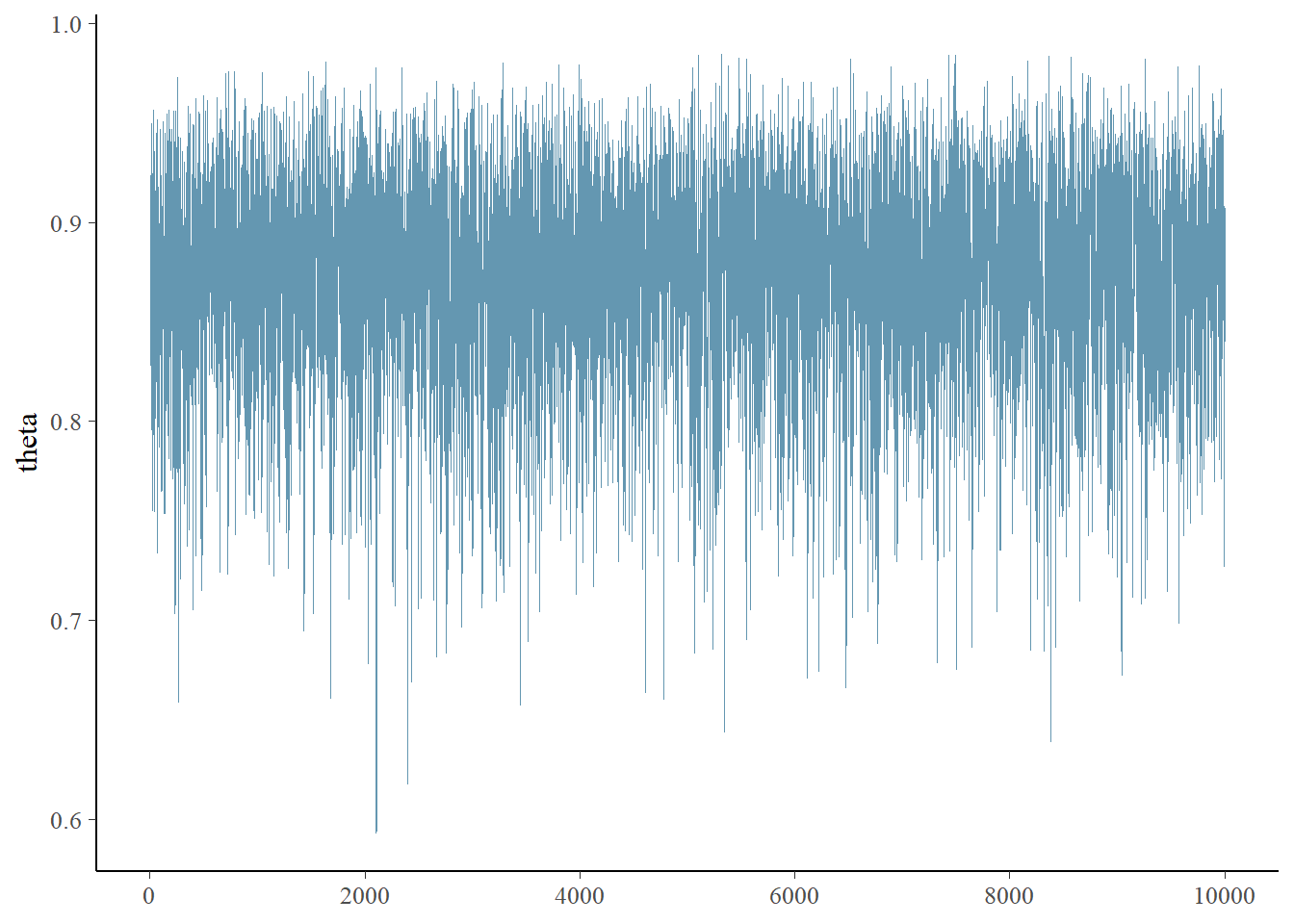
10.1.6 Posterior prediction
The output from coda.samples is stored as an mcmc.list format. The simulated values of the variables identified in the variable.names argument can be extracted as a matrix (or array) and then manipulated as usual R objects.
thetas = as.matrix(posterior_sample)
head(thetas)
## theta
## [1,] 0.8405
## [2,] 0.8284
## [3,] 0.9183
## [4,] 0.9114
## [5,] 0.9238
## [6,] 0.9010hist(thetas)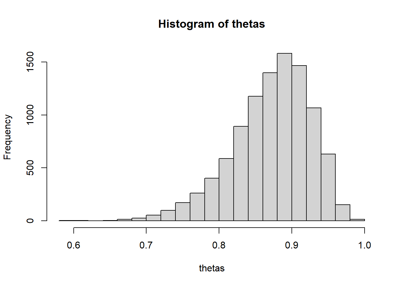
The matrix would have one column for each variable named in variable.names; in this case, there is only one column corresponding to the simulated values of theta.
We can now use the simulated values of theta to simulate replicated samples to approximate the posterior predictive distribution. To be clear, the code below is running R commands within R (not JAGS).
(There is a way to simulate predictive values within JAGS itself, but I think it’s more straightforward in R. Just use JAGS to get a simulated sample from the posterior distribution. On the other hand, if you’re using Stan there are functions for simulating and summarizing posterior predicted values.)
ynew = rbinom(Nrep, n, thetas)

plot(table(ynew),
     main = "Posterior Predictive Distribution for samples of size 35",
     xlab = "y")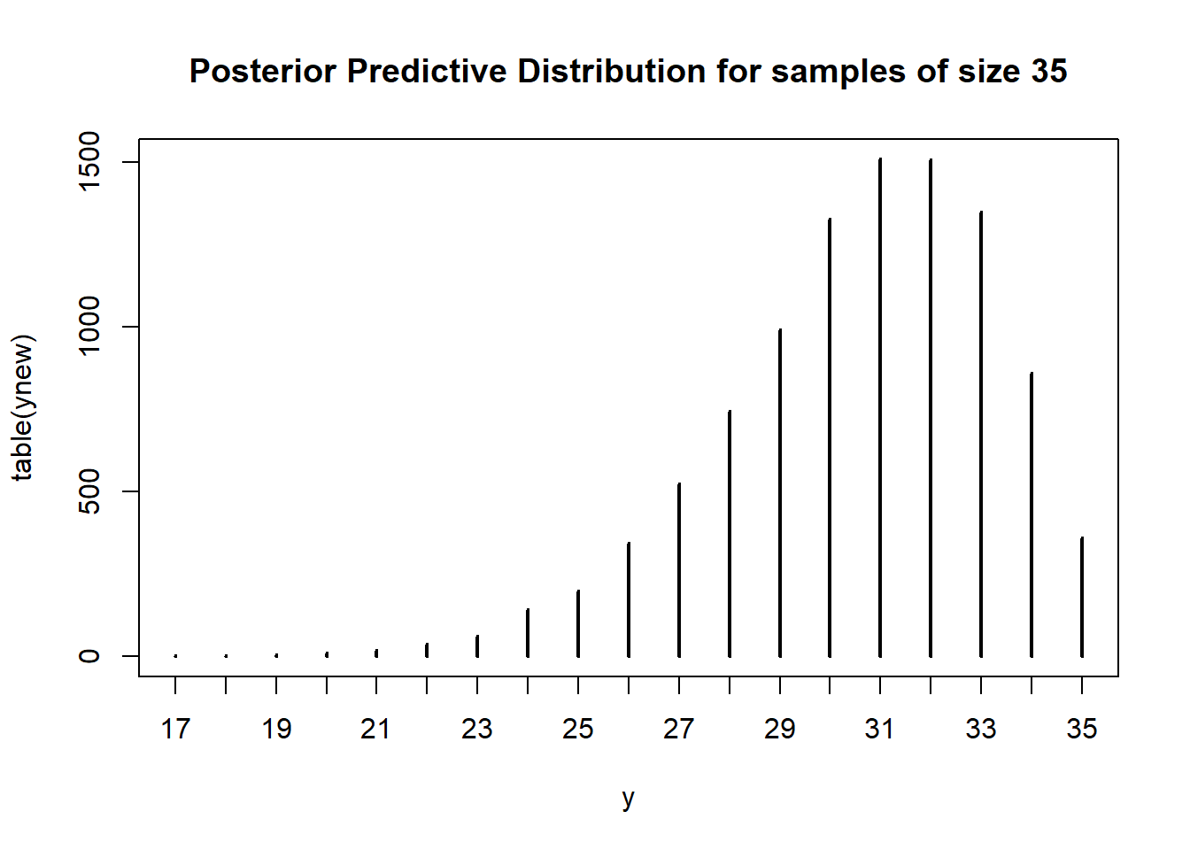
10.1.7 Loading data as individual values rather than summary statistics
Instead of the total count (modeled by a Binomial likelihood), the individual data values (1/0 = S/F) can be provided, which could be modeled by a Bernoulli (i.e. Binomial(trials=1)) likelihood. That is, \((Y_1, \ldots, Y_n|\theta)\sim\) i.i.d. Bernoulli(\(\theta\)), rather than \((Y|\theta)\sim\) Binomial\((n, \theta)\). The vector y below represents the data in this format. Notice how the likelihood in the model specification changes in response; the n observations are specified via a for loop.
# Load the data
y = c(rep(1, 31), rep(0, 4)) # vector of 31 1s and 4 0s
n = length(y)

model_string <- "model{

  # Likelihood
  for (i in 1:n){
    y[i] ~ dbern(theta)
  }

  # Prior
  theta ~ dbeta(alpha, beta)
  alpha <- 3
  beta <- 1

}"
10.1.8 Simulating multiple chains
The Bernoulli model can be passed to JAGS similar to the Binomial model above. Below, we have also introduced the n.chains argument, which simulates multiple Markov chains and allows for some additional diagnostic checks. Simulating multiple chains helps assess convergence of the Markov chain to the target distribution. (We’ll discuss more details later.) Initial values for the chains can be provided in a list with the inits argument; otherwise initial values are generated automatically.
# Compile the model
dataList = list(y = y, n = n)

model <- jags.model(textConnection(model_string),
                    data = dataList,
                    n.chains = 5)
## Compiling model graph
## Resolving undeclared variables
## Allocating nodes
## Graph information:
## Observed stochastic nodes: 35
## Unobserved stochastic nodes: 1
## Total graph size: 39
##
## Initializing model# Simulate
update(model, 1000, progress.bar = "none")
Nrep = 10000
posterior_sample <- coda.samples(model,
variable.names = c("theta"),
n.iter = Nrep,
progress.bar = "none")
# Summarize and check diagnostics
summary(posterior_sample)##
## Iterations = 1001:11000
## Thinning interval = 1
## Number of chains = 5
## Sample size per chain = 10000
##
## 1. Empirical mean and standard deviation for each variable,
## plus standard error of the mean:
##
## Mean SD Naive SE Time-series SE
## 0.871900 0.052849 0.000236 0.000235
##
## 2. Quantiles for each variable:
##
## 2.5% 25% 50% 75% 97.5%
## 0.753 0.840 0.878 0.911 0.956plot(posterior_sample)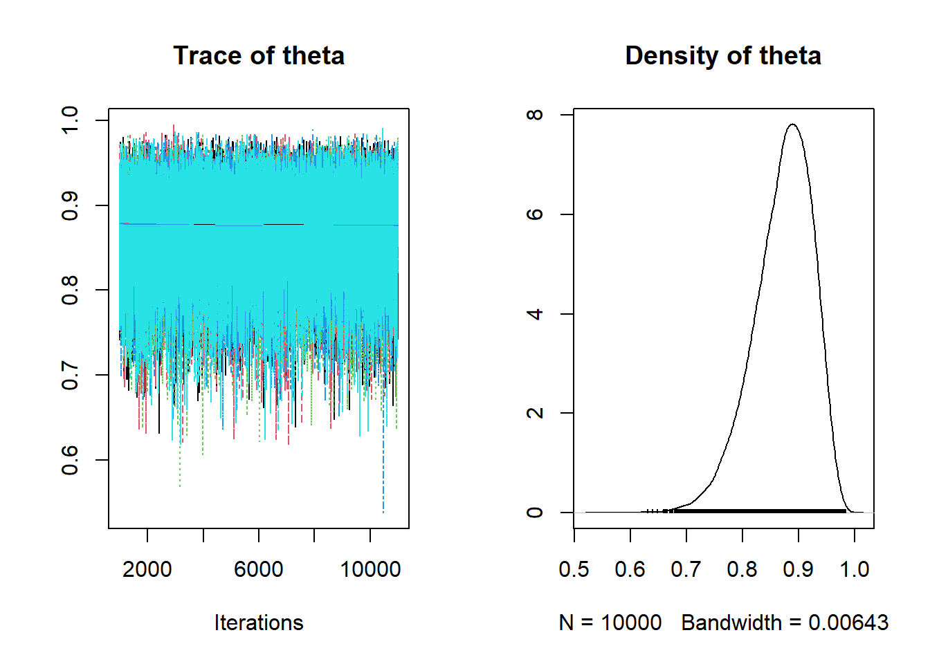
If multiple chains are simulated, the DBDA2E function diagMCMC can be used for diagnostics.
Note: Some of the DBDA2E output, in particular from diagMCMC, isn’t always displayed when the RMarkdown file is knit. You might need to manually run these cells within RStudio. I’m not sure why; please let me know if you figure it out.
plotPost(posterior_sample)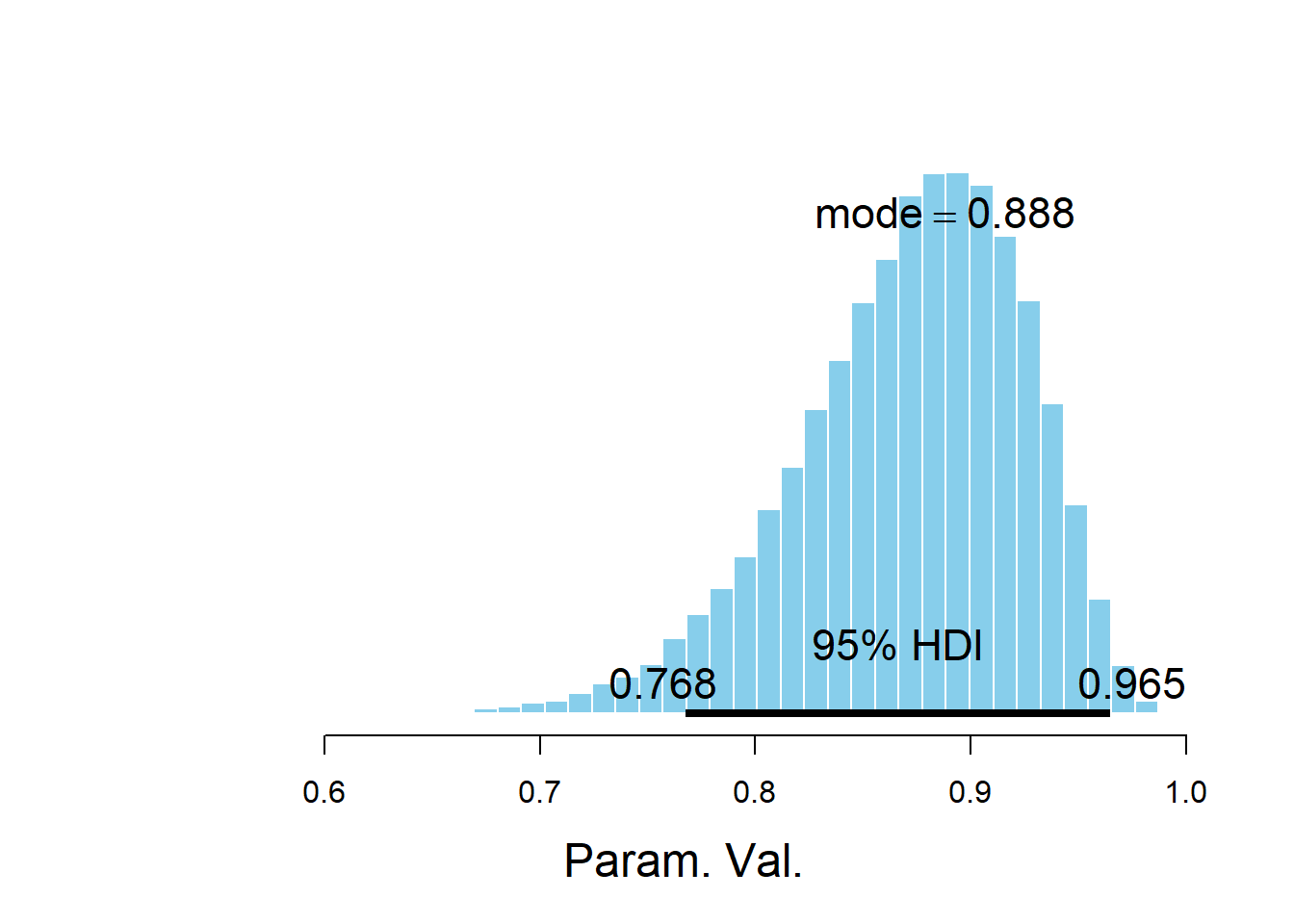
##               ESS   mean median   mode hdiMass hdiLow hdiHigh compVal
## Param. Val. 50000 0.8719 0.8784 0.8882    0.95 0.7676  0.9649      NA
##             pGtCompVal ROPElow ROPEhigh pLtROPE pInROPE pGtROPE
## Param. Val. NA NA NA NA NA NAdiagMCMC(posterior_sample)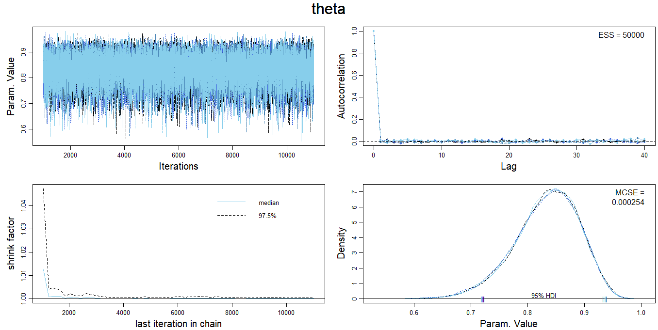
10.1.9 ShinyStan
We can use regular R functionality for plotting, or functions from packages likes DBDA2E or bayesplot. Another nice tool is ShinyStan, which provides an interactive utility for exploring the results of MCMC simulations. While ShinyStan was developed for the Stan package, it can use output from JAGS and other MCMC packages. You’ll need to install the shinystan package and its dependencies.
The code below will launch in a browser the ShinyStan GUI for exploring the results of the JAGS simulation. The as.shinystan command takes coda.samples output (stored as an mcmc-list) and puts it in the proper format for ShinyStan. (Note: this code won’t display anything in the notes. You’ll have to actually run it to see what happens.)
library(shinystan)
my_sso <- launch_shinystan(as.shinystan(posterior_sample,
                                        model_name = "Bortles!!!"))
10.1.10 Back to the left-handed problem
Let’s return again to the problem in Example 10.1, in which we wanted to estimate the proportion of Cal Poly students that are left-handed. Assume a Normal distribution prior for \(\theta\) with mean 0.15 and SD 0.08. Also suppose that in a sample of 25 Cal Poly students 5 are left-handed. We will use JAGS to find the (approximate) posterior distribution.
Important note: in JAGS a Normal distribution is parametrized by its precision, which is the reciprocal of the variance: dnorm(mean, precision). That is, for a \(N(\mu,\sigma)\) distribution, the precision, often denoted \(\tau\), is \(\tau = 1/\sigma^2\). For example, in JAGS dnorm(0, 1 / 4) corresponds to a precision of 1/4, a variance of 4, and a standard deviation of 2.
# Data
n = 25
y = 5

# Model
model_string <- "model{

  # Likelihood
  y ~ dbinom(theta, n)

  # Prior
  theta ~ dnorm(mu, tau)
  mu <- 0.15 # prior mean
  tau <- 1 / 0.08 ^ 2 # prior precision; prior SD = 0.08

}"

dataList = list(y = y, n = n)

# Compile
model <- jags.model(file = textConnection(model_string),
                    data = dataList)
## Compiling model graph
## Resolving undeclared variables
## Allocating nodes
## Graph information:
## Observed stochastic nodes: 1
## Unobserved stochastic nodes: 1
## Total graph size: 9
##
## Initializing modelmodel <- jags.model(textConnection(model_string),
data = dataList,
n.chains = 5)## Compiling model graph
## Resolving undeclared variables
## Allocating nodes
## Graph information:
## Observed stochastic nodes: 1
## Unobserved stochastic nodes: 1
## Total graph size: 9
##
## Initializing model# Simulate
update(model, 1000, progress.bar = "none")
Nrep = 10000
posterior_sample <- coda.samples(model,
variable.names = c("theta"),
n.iter = Nrep,
progress.bar = "none")
# Summarize and check diagnostics
summary(posterior_sample)##
## Iterations = 2001:12000
## Thinning interval = 1
## Number of chains = 5
## Sample size per chain = 10000
##
## 1. Empirical mean and standard deviation for each variable,
## plus standard error of the mean:
##
## Mean SD Naive SE Time-series SE
## 0.183316 0.051952 0.000232 0.000293
##
## 2. Quantiles for each variable:
##
## 2.5% 25% 50% 75% 97.5%
## 0.0888 0.1465 0.1807 0.2176 0.2909plot(posterior_sample)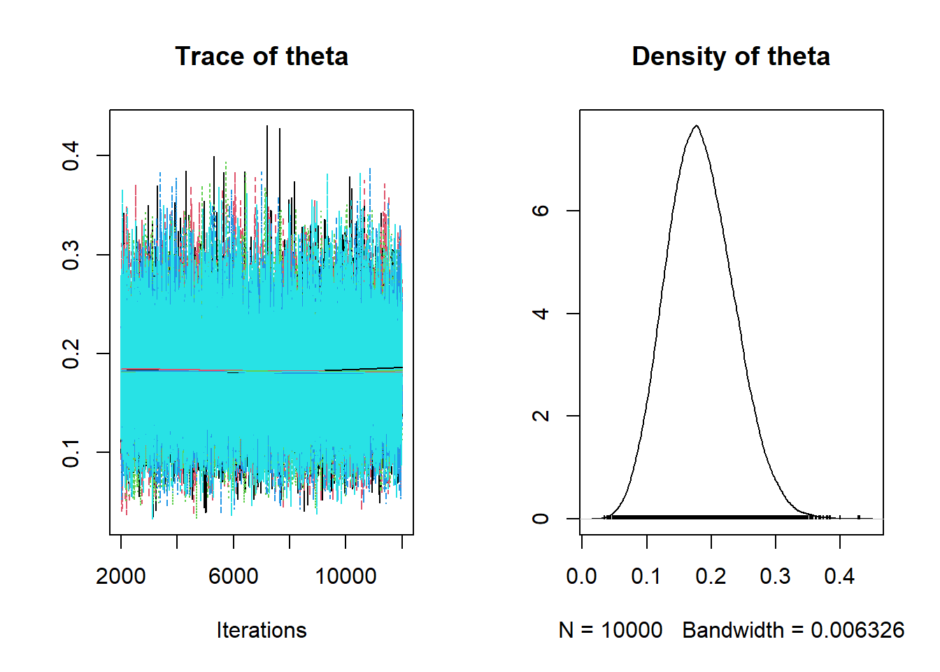
The posterior density is similar to what we computed with the grid approximation.