Chapter 14 Introduction to Multi-Parameter Models
So far we have considered situations with a just a single unknown parameter \(\theta\). However, most interesting problems involve multiple unknown parameters.
For example, we have considered the problem of estimating the population mean of a numerical variable assuming the population standard deviation was known. However, in practice both the population mean and population standard deviation are unknown. Even if we are only interested in estimating the population mean, we still need to account for the uncertainty in the population standard deviation.
When there are two (or more) unknown parameters the prior and posterior distribution will each be a joint probability distribution over pairs (or tuples/vectors) of possible values of the parameters.
Example 14.1 Assume body temperatures (degrees Fahrenheit) of healthy adults follow a Normal distribution with unknown mean \(\mu\) and unknown standard deviation \(\sigma\). Suppose we wish to estimate both \(\mu\), the population mean healthy human body temperature, and \(\sigma\), the population standard deviation of body temperatures.
Assume a discrete prior distribution according to which
- \(\mu\) takes values 97.6, 98.1, 98.6 with prior probability 0.2, 0.3, 0.5, respectively.
- \(\sigma\) takes values 0.5, 1 with prior probability 0.25, 0.75, respectively.
- \(\mu\) and \(\sigma\) are independent.
Start to construct the Bayes table. What are the possible values of the parameter? What are the prior probabilities? (Hint: the parameter \(\theta\) is a pair \((\mu, \sigma)\).)
Suppose two temperatures of 97.5 and 97.9 are observed, independently. Identify the likelihood.
Complete the Bayes table and find the posterior distribution after observing these two measurements. Compare to the prior distribution.
Suppose that we only observe that in a sample of size 2 the mean is 97.7. Is this information enough to evaluate the likelihood function and determine the posterior distribution?
The prior assumes that \(\mu\) and \(\sigma\) are independent. Are they independent according to the posterior distribution?
See the table below. There are 3 possible values for \(\mu\) and 2 possible values for \(\sigma\) so there are \((3)(2)=6\) possible \((\mu, \sigma)\) pairs. Each row in the Bayes table represents a \((\mu, \sigma)\) pair. Since the prior assumes independence, the prior probability of any pair is the product of the marginal prior probabilities of \(\mu\) and \(\sigma\). For example, the probability probability that \(\mu = 97.6\) and \(\sigma=0.5\) is \((0.2)(0.25)=0.05\)
The likelihood is similar to what we have seen in other examples concerning body temperature, but it is now a function of both \(\mu\) and \(\sigma\). That is, the likelihood is a function of two variables. The likelihood is determined by evaluating, for each \((\mu, \sigma)\) pair, the Normal(\(\mu\), \(\sigma\)) density at each of \(y=97.9\) and \(y=97.5\) and then finding the product: \[ {\scriptstyle f(y=(97.9, 97.5)|\mu, \sigma) \propto \left[\sigma^{-1}\,\exp\left(-\frac{1}{2}\left(\frac{97.9-\mu}{\sigma}\right)^2\right)\right]\left[\sigma^{-1}\,\exp\left(-\frac{1}{2}\left(\frac{97.5-\mu}{\sigma}\right)^2\right)\right] } \]
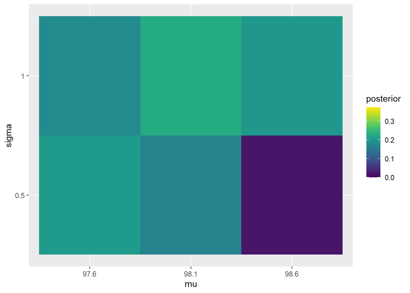
See the table below. As always, posterior is proportional to likelihood times prior. For the sample (97.9, 97.5), the sample mean is 97.7 and the sample standard deviation is 0.283. The posterior distribution pushes probability away from \(\mu=98.6\), and pushes more probability towards \(\sigma=0.5\).
mu = c(97.6, 98.1, 98.6)
sigma = c(0.5, 1)
theta = expand.grid(mu, sigma) # all possible (mu, sigma) pairs
names(theta) = c("mu", "sigma")

# prior

prior_mu = c(0.20, 0.30, 0.50)
prior_sigma = c(0.25, 0.75)
prior = apply(expand.grid(prior_mu, prior_sigma), 1, prod)
prior = prior / sum(prior)

# data
y = c(97.9, 97.5) # single observed value

# likelihood
likelihood = dnorm(97.9, mean = theta$mu, sd = theta$sigma) *
  dnorm(97.5, mean = theta$mu, sd = theta$sigma)

# posterior
product = likelihood * prior
posterior = product / sum(product)

# bayes table
bayes_table = data.frame(theta,
                     prior,
                     likelihood,
                     product,
                     posterior)

kable(bayes_table, digits = 4, align = 'r')
mu sigma prior likelihood product posterior 97.6 0.5 0.050 0.5212 0.0261 0.2041 98.1 0.5 0.075 0.2861 0.0215 0.1680 98.6 0.5 0.125 0.0212 0.0027 0.0208 97.6 1.0 0.150 0.1514 0.0227 0.1778 98.1 1.0 0.225 0.1303 0.0293 0.2296 98.6 1.0 0.375 0.0680 0.0255 0.1997 Intuitively, knowing only the posterior mean would not be sufficient, since it would not give us enough information to estimate the standard deviation \(\sigma\). In order to evaluate the likelihood we need to compute \(\frac{y-\mu}{\sigma}\) for each individual \(y\) value, so if we only had the sample mean we would not be able to fill in the likelihood column.
The posterior distribution represents some dependence between \(\mu\) and \(\sigma\). For example, consider the pair \(\mu=97.6\) and \(\sigma=0.5\). The marginal posterior probability that \(\mu=97.6\) is 0.3819. The marginal posterior probability that \(\sigma=0.5\) is 0.3929. But the joint posterior probability that \(\mu=97.6\) and \(\sigma=0.5\) is 0.2041, which is not the product of the marginal probabilities.
The plots below compare the prior and posterior distributions from the previous problem.
ggplot(bayes_table %>%
         mutate(mu = factor(mu),
                sigma = factor(sigma)),
       aes(mu, sigma)) +
    geom_tile(aes(fill = prior))  +
  scale_fill_viridis(limits = c(0, max(c(prior, posterior))))

ggplot(bayes_table %>%
         mutate(mu = factor(mu),
                sigma = factor(sigma)),
       aes(mu, sigma)) +
    geom_tile(aes(fill = posterior)) +
  scale_fill_viridis(limits = c(0, max(c(prior, posterior))))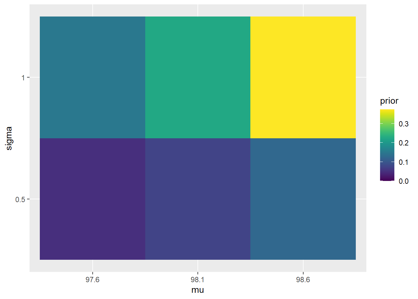
Example 14.2 Continuing Example 14.1, let’s assume a more reasonable, continuous prior for \((\mu,\sigma)\). We have seen that we often work with the precision \(\tau = 1/\sigma^2\) rather than the SD. Assume a continuous prior distribution which assumes
- \(\mu\) has a Normal distribution with mean 98.6 and standard deviation 0.3.
- \(\tau\) has a Gamma distribution with shape parameter 5 and rate parameter 2.
- \(\mu\) and \(\tau\) are independent.
(This problem just concerns the prior distribution. We’ll look at this posterior distribution in the next example.)
- Simulate \((\mu, \tau)\) pairs from the prior distribution and plot them.
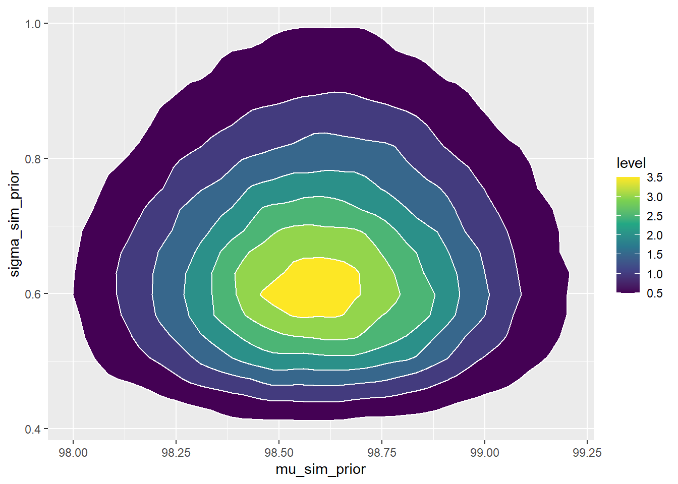
- Simulate \((\mu, \sigma)\) pairs from the prior distribution and plot them. Describe the prior distribution of \(\sigma\).
- Find and interpret a central 98% prior credible interval for \(\mu\).
- Find a central 98% prior credible interval for the precision \(\tau=1/\sigma^2\).
- Find and interpret a central 98% prior credible interval for \(\sigma\).
- What is the prior credibility that both \(\mu\) and \(\sigma\) lie within their credible intervals?
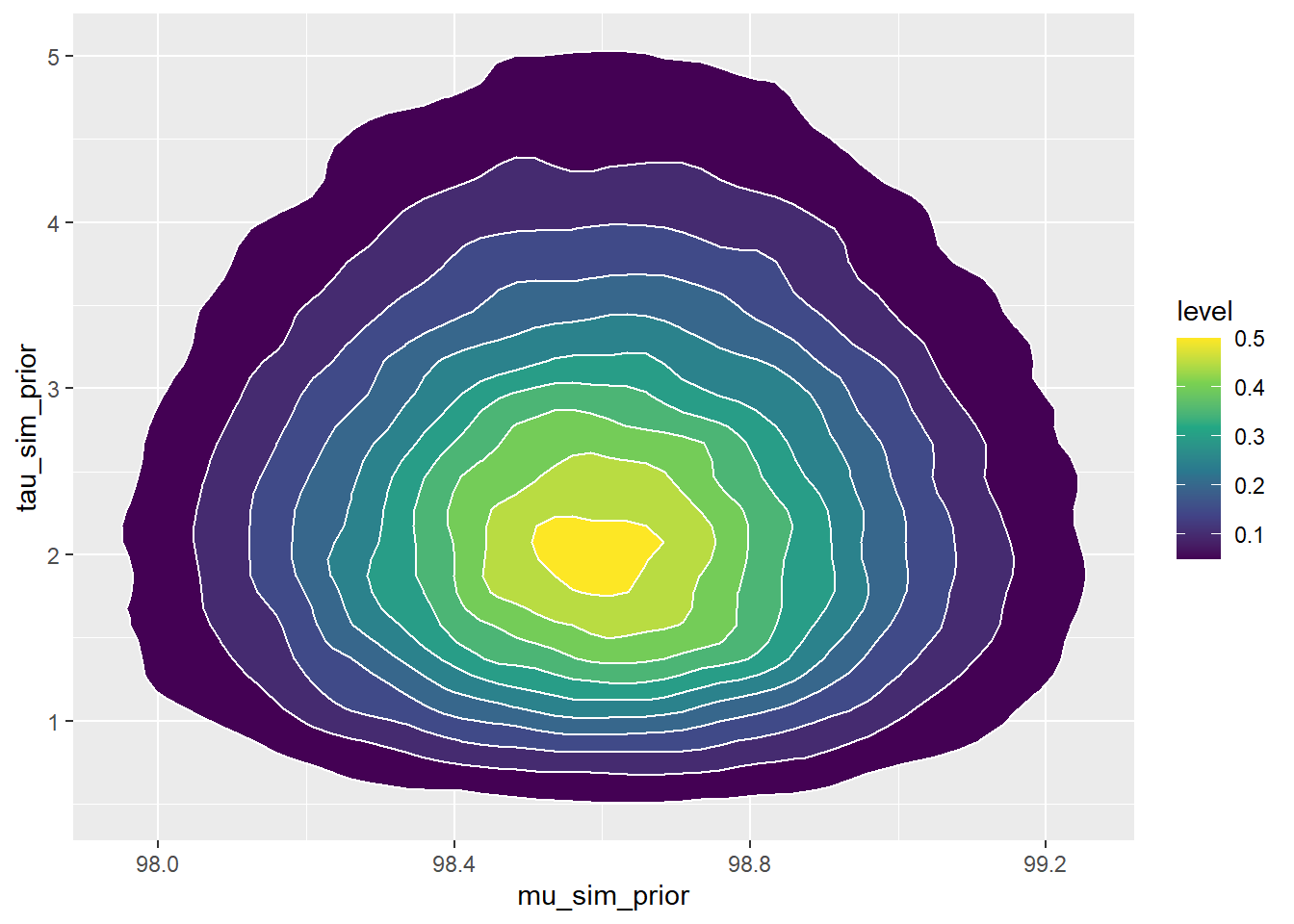
We could plot the prior distribution directly. However, distributions are usually only approximated via simulation, so we’ll just simulate. The prior distribution is a distribution on \((\mu,\tau)\) pairs.
Nrep = 100000

mu_sim_prior = rnorm(Nrep, 98.6, 0.3)
tau_sim_prior = rgamma(Nrep, shape = 5, rate = 2)
sigma_sim_prior = 1 / sqrt(tau_sim_prior)
sim_prior = data.frame(mu_sim_prior, tau_sim_prior, sigma_sim_prior)

ggplot(sim_prior, aes(mu_sim_prior, tau_sim_prior)) +
  geom_point(color = "skyblue", alpha = 0.4)

ggplot(sim_prior, aes(mu_sim_prior, tau_sim_prior)) +
  stat_density_2d(aes(fill = ..level..),
              geom = "polygon", color = "white") +
 scale_fill_viridis_c()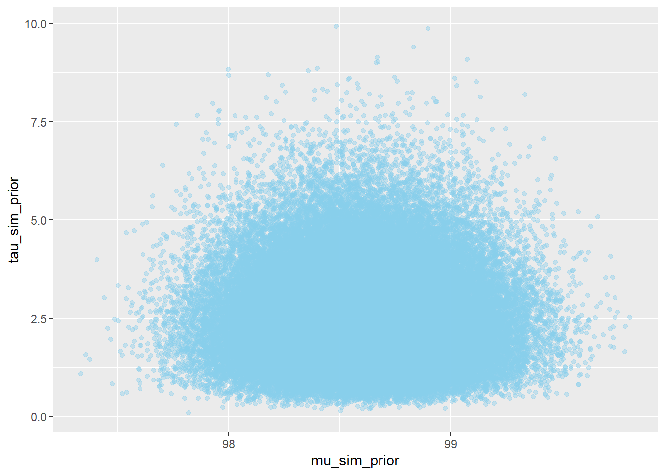
See plots below. The prior distribution on \(\tau\) induces a prior distribution on \(\sigma = 1/\sqrt{\tau}\).
ggplot(sim_prior, aes(x = sigma_sim_prior)) +
 geom_histogram(aes(y=..density..), color = "black", fill = "white") +
 geom_density(size = 1, color = "skyblue")

ggplot(sim_prior, aes(mu_sim_prior, sigma_sim_prior)) +
  stat_density_2d(aes(fill = ..level..),
              geom = "polygon", color = "white") +
 scale_fill_viridis_c()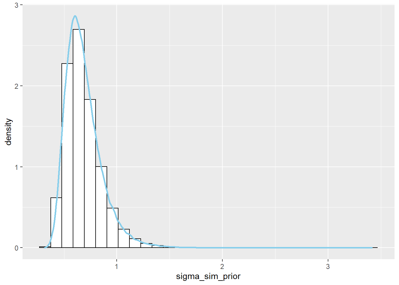
There is a prior probability of 98% that population mean human body temperature is between 97.9 and 99.3 degrees F.
quantile(mu_sim_prior, c(0.01, 0.99))## 1% 99% ## 97.9 99.3We can compute a credible interval like usual. Precision just doesn’t have as practical an interpretation as standard deviation.
quantile(tau_sim_prior, c(0.01, 0.99))## 1% 99% ## 0.6374 5.8224There is a prior probability of 98% that population standard deviation of human body temperatures is between 0.41 and 1.25 degrees F.
quantile(sigma_sim_prior, c(0.01, 0.99))## 1% 99% ## 0.4144 1.2526Since \(\mu\) and \(\sigma\) are independent according to the prior distribution, the probability that both parameters lie in their respective intervals is (0.98)(0.98)=0.9604. If we want 98% joint prior credibility, we need a different region.
Example 14.3 Continuing the previous example, we’ll now compute the posterior distribution given a sample of two measurements of 97.9 and 97.5.
- Assume a grid of \(\mu\) values from 96.0 to 100.0 in increments of 0.01, and a grid of \(\tau\) values from 0.1 to 25.0 in increments of 0.01. How many possible values of the pair \((\mu, \tau)\) are there; that is, how many rows are there in the Bayes table?
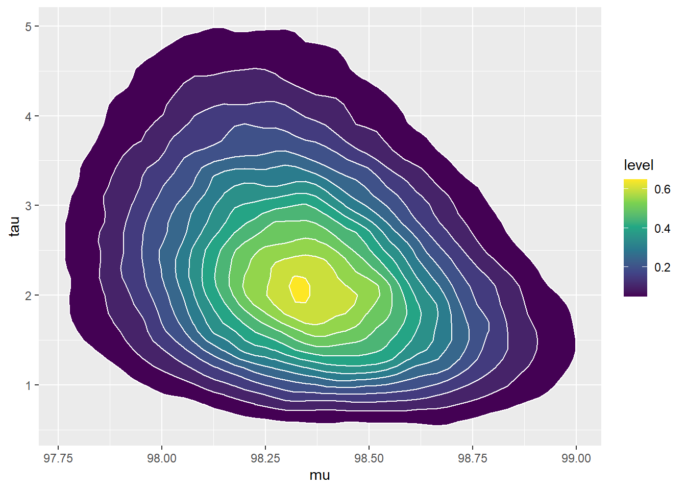
- Use grid approximation to approximate the joint posterior distribution of \((\mu, \tau)\) Simulate values from the joint posterior distribution and plot them. Compute the posterior correlation between \(\mu\) and \(\tau\); are they independent according to the posterior distribution?
- Plot the simulated joint posterior distribution of \(\mu\) and \(\sigma\). Compare to the prior.
- Suppose we wanted to approximate the posterior distribution without first using grid approximation. Describe how, in principle, you would use a naive (non-MCMC) simulation to approximate the posterior distribution. In practice, what is the problem with such a simulation?
There are (100-96)/0.01 = 400 values of \(\mu\) in the grid (actually 401 including both endpoints) and (25-0.1)/0.01 = 2490 values of \(\mu\) in the grid (actually 2491). There are almost 1 million possible values of the pair \((\mu, \tau)\) in the grid.
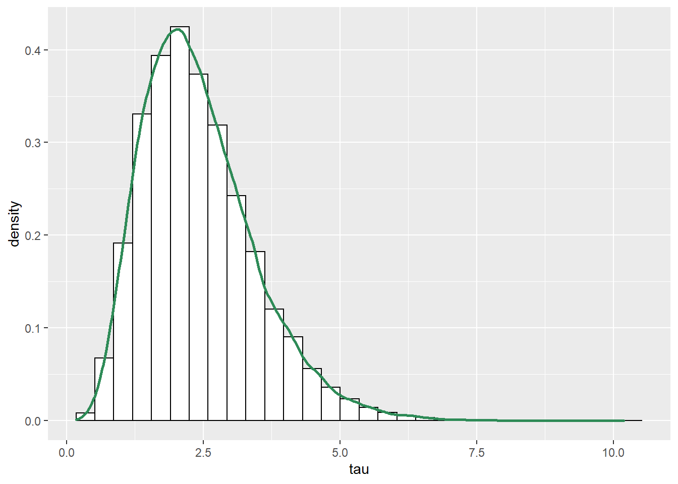
See below. Even though \(\mu\) and \(\tau\) are independent according to the prior distribution, there is a negative posterior correlation. (Below the posterior is computed via grid approximation. After the posterior distribution was computed, values were simulated from it for plotting.)
# parameters
mu = seq(96.0, 100.0, 0.01)
tau = seq(0.1, 25, 0.01)

theta = expand.grid(mu, tau)
names(theta) = c("mu", "tau")
theta$sigma = 1 / sqrt(theta$tau)

# prior
prior_mu_mean = 98.6
prior_mu_sd = 0.3

prior_precision_shape = 5
prior_precision_rate = 2

prior = dnorm(theta$mu, prior_mu_mean, sd = prior_mu_sd) *
  dgamma(theta$tau, shape = prior_precision_shape,
                     rate = prior_precision_rate)
prior = prior / sum(prior)

# data
y = c(97.9, 97.5)

# likelihood
likelihood = dnorm(97.9, mean = theta$mu, sd = theta$sigma) *
  dnorm(97.5, mean = theta$mu, sd = theta$sigma)

# posterior
product = likelihood * prior
posterior = product / sum(product)

# posterior simulation
sim_posterior = theta[sample(1:nrow(theta), 100000, replace = TRUE, prob = posterior), ]

cor(sim_posterior$mu, sim_posterior$tau)
## [1] -0.2888#plots ggplot(sim_posterior, aes(mu)) + geom_histogram(aes(y=..density..), color = "black", fill = "white") + geom_density(size = 1, color = "seagreen") ggplot(sim_posterior, aes(tau)) + geom_histogram(aes(y=..density..), color = "black", fill = "white") + geom_density(size = 1, color = "seagreen") ggplot(sim_posterior, aes(mu, tau)) + stat_density_2d(aes(fill = ..level..), geom = "polygon", color = "white") + scale_fill_viridis_c()
See below. We see that the posterior shifts the density towards smaller values of \(\mu\) and \(\sigma\). There is also a slight positive posterior correlation between \(\mu\) and \(\sigma\).
cor(sim_posterior$mu, sim_posterior$sigma)## [1] 0.2804#plots ggplot(sim_posterior, aes(mu)) + geom_histogram(aes(y=..density..), color = "black", fill = "white") + geom_density(size = 1, color = "seagreen") ggplot(sim_posterior, aes(sigma)) + geom_histogram(aes(y=..density..), color = "black", fill = "white") + geom_density(size = 1, color = "seagreen") ggplot(sim_posterior, aes(mu, sigma)) + stat_density_2d(aes(fill = ..level..), geom = "polygon", color = "white") + scale_fill_viridis_c()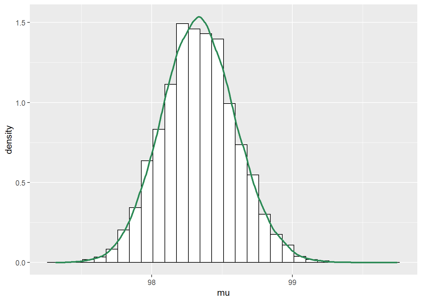
Simulate a value of \((\mu, \sigma)\) from their joint prior distribution, by simulating a value of \(\mu\) from a Normal(98.6, 0.3) distribution and simulating, independently, a value of \(\tau\) from a Gamma(5, 2) distribution and setting \(\sigma = 1/\sqrt{\tau}\). Given \(\mu\) and \(\sigma\) simulate two independent \(y\) values from a Normal(\(\mu\), \(\sigma\)) distribution. Repeat many times. Condition on the observed data by discarding any repetitions for which the \(y\) values are not (97.9, 97.5), to some reasonable degree of precision, say rounded to 1 decimal place. Approximate the posterior distribution using the remaining simulated values of \((\mu, \sigma)\).
In practice, the probability of seeing a sample with \(y\) values of 97.9 and 97.5 is extremely small, so almost all repetitions of the simulation would be discarded and such a simulation would be extremely computationally inefficient. (For example, the values of \(\mu\) and \(\sigma\) which maximize the likelihood of (97.9, 97.5) are 97.7 and 0.2, respectively, and even for those values and rounding to 1 decimal place the probability of seeing such a sample is only 0.015.)
The previous problem illustrates that grid approximation can quickly become computationally infeasible when there are multiple parameters (to obtain sufficient precision). Naively conditioning a simulation on the observed sample is also computationally infeasible, since except in the simplest situations the probability of recreating the observed sample in a simulation is essentially 0. Therefore, we need more efficient computational methods, and MCMC will do the trick.
temperature data file contains 208 measurements of human body temperature (degrees F).
The sample mean is 97.71 degrees F and the sample SD is 0.75 degrees F.
Assuming the same prior distribution as in the previous problem, use JAGS to approximate the joint posterior distribution of \(\mu\) and \(\sigma\).
Summarize the posterior distribution in context.
The JAGS code is below. A few comments on the code
- The data is read as individual values, so the likelihood of each
y[i]is computed via a for loop. - We have called the parameters by their names
mu,tau,sigma, rather than just a singletheta. - We specify a prior distribution on
tauand then definesigma <- 1 / sqrt(tau). - In JAGS
dnormis of the formdnorm(mean, precision) - We are interested in the posterior distribution of \(\mu\) and \(\sigma\), so we include both parameters in the
model.namesargument of thecoda.samplesfunction. - The output of
coda.samplesis a special object called anmcmc.list. Callingploton this object produces a trace plot and a density plot for each parameter included invariable.names. But it does not automatically produce any joint distribution plots. - We use
mcmc_scatterfrom thebayesplotpackage to create a scatter plot of the joint posterior distribution, to which we can add contours. - We can also extract the JAGS output as a matrix, put it in a data frame, and then use R or ggplot commands to create plots.
- The simulated values from an
mcmc.listcan be extracted as a matrix withas.matrixand then manipulated as usual, e.g., to compute the correlation.
Nrep = 10000
Nchains = 3

# data
data = read.csv("_data/temperature.csv")
y = data$temperature
n = length(y)

# model
model_string <- "model{

  # Likelihood
  for (i in 1:n){
    y[i] ~ dnorm(mu, 1 / sigma ^ 2)
  }

  # Prior
  mu ~ dnorm(98.6, 1 / 0.3 ^ 2)

  sigma <- 1 / sqrt(tau)
  tau ~ dgamma(5, 2)

}"

# Compile the model
dataList = list(y=y, n=n)

model <- jags.model(textConnection(model_string),
                    data=dataList,
                    n.chains=Nchains)
## Compiling model graph
## Resolving undeclared variables
## Allocating nodes
## Graph information:
## Observed stochastic nodes: 208
## Unobserved stochastic nodes: 2
## Total graph size: 222
##
## Initializing modelupdate(model, 1000, progress.bar="none")
posterior_sample <- coda.samples(model,
variable.names=c("mu", "sigma"),
n.iter=Nrep,
progress.bar="none")
# Summarize and check diagnostics
summary(posterior_sample)##
## Iterations = 2001:12000
## Thinning interval = 1
## Number of chains = 3
## Sample size per chain = 10000
##
## 1. Empirical mean and standard deviation for each variable,
## plus standard error of the mean:
##
## Mean SD Naive SE Time-series SE
## mu 97.737 0.0513 0.000296 0.000296
## sigma 0.749 0.0358 0.000207 0.000264
##
## 2. Quantiles for each variable:
##
## 2.5% 25% 50% 75% 97.5%
## mu 97.637 97.702 97.737 97.771 97.837
## sigma 0.684 0.724 0.748 0.773 0.823plot(posterior_sample)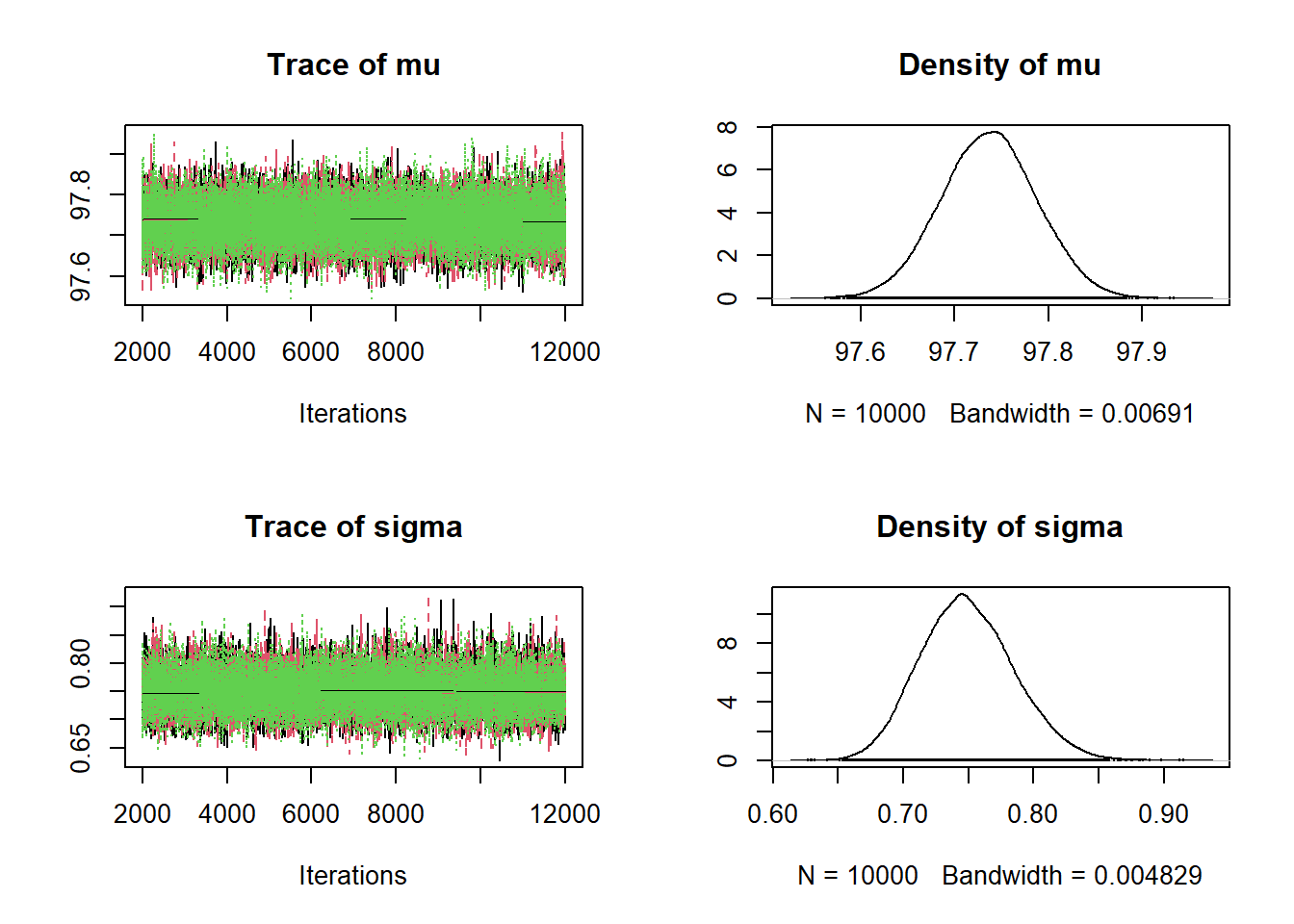
# Scatterplot from bayesplot package
color_scheme_set("green")
mcmc_scatter(posterior_sample, pars = c("mu", "sigma"), alpha = 0.1) +
  stat_ellipse(level = 0.98, color = "black", size = 2) +
  stat_density_2d(color = "grey", size = 1)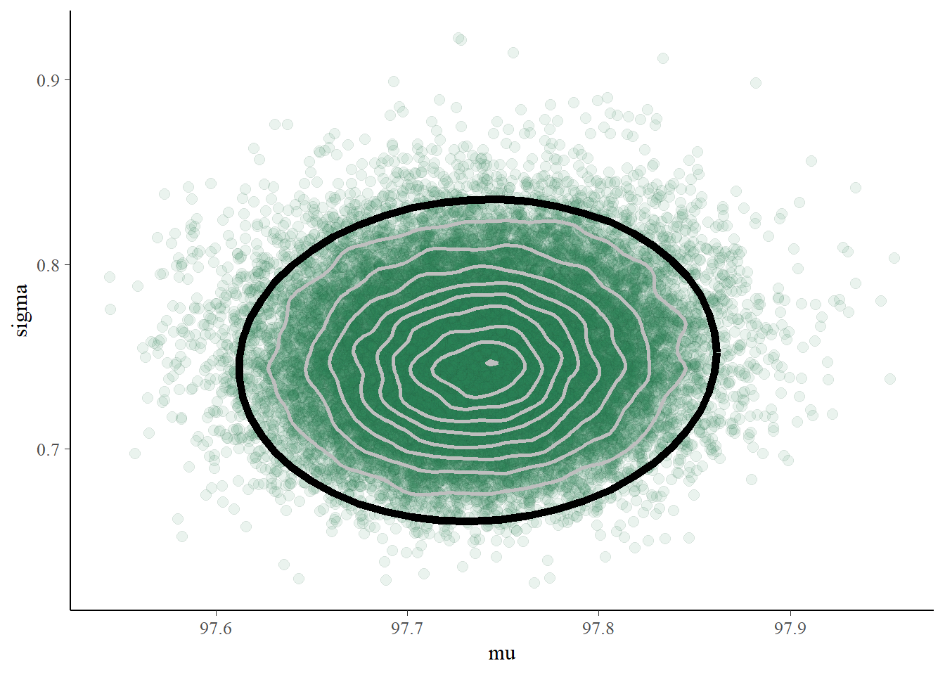
# posterior summary
posterior_sim = data.frame(as.matrix(posterior_sample))

head(posterior_sim)
## mu sigma
## 1 97.74 0.7825
## 2 97.66 0.7844
## 3 97.75 0.8094
## 4 97.75 0.7028
## 5 97.79 0.6983
## 6 97.73 0.8027apply(posterior_sim, 2, mean)## mu sigma
## 97.7368 0.7493apply(posterior_sim, 2, sd)## mu sigma
## 0.05125 0.03581quantile(posterior_sim$mu, c(0.01, 0.99))## 1% 99%
## 97.62 97.86quantile(posterior_sim$sigma, c(0.01, 0.99))## 1% 99%
## 0.6732 0.8377cor(posterior_sim)## mu sigma
## mu 1.00000 0.04892
## sigma 0.04892 1.00000ggplot(posterior_sim, aes(mu)) +
geom_histogram(aes(y=..density..), color = "black", fill = "white") +
geom_density(size = 1, color = "seagreen")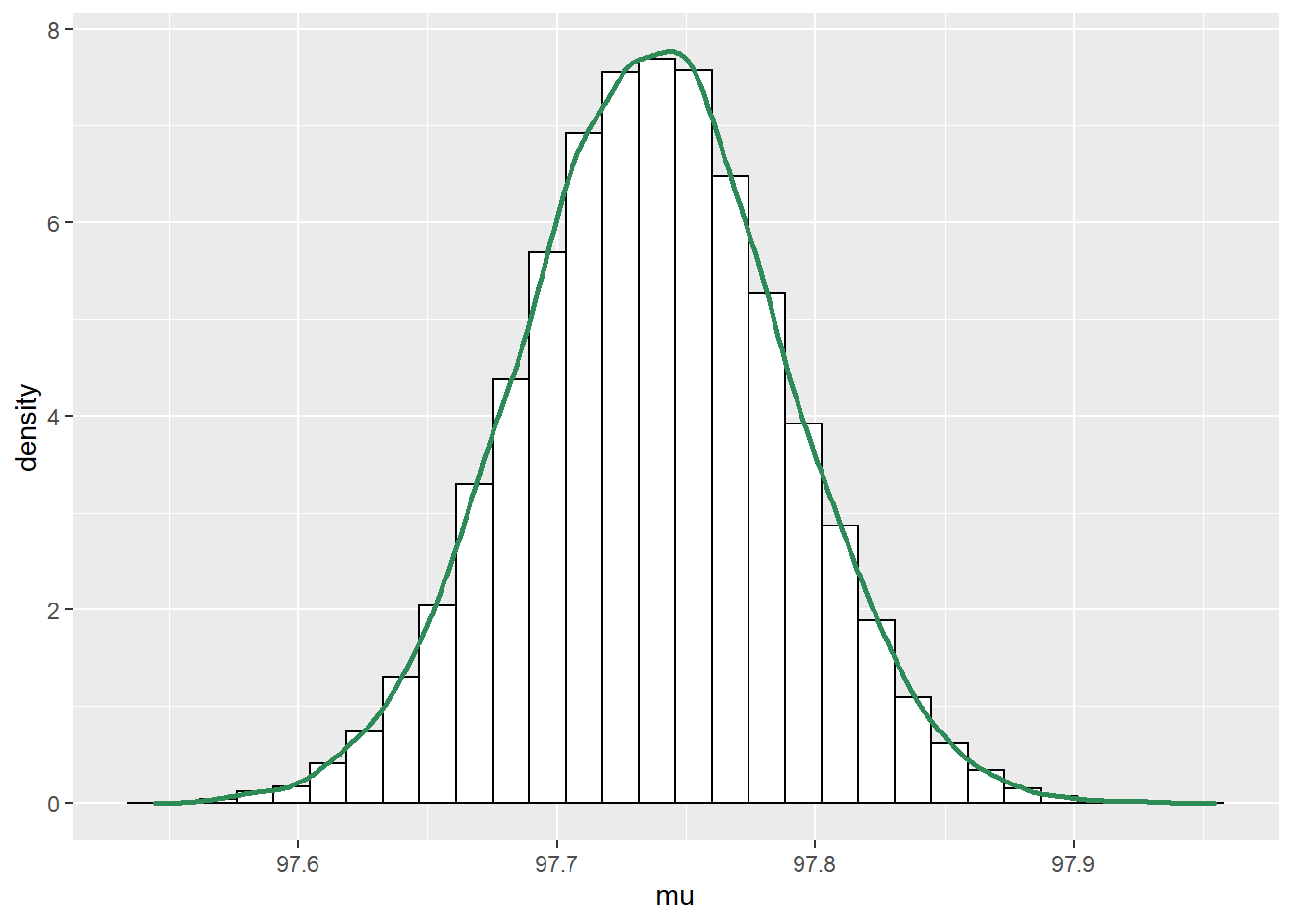
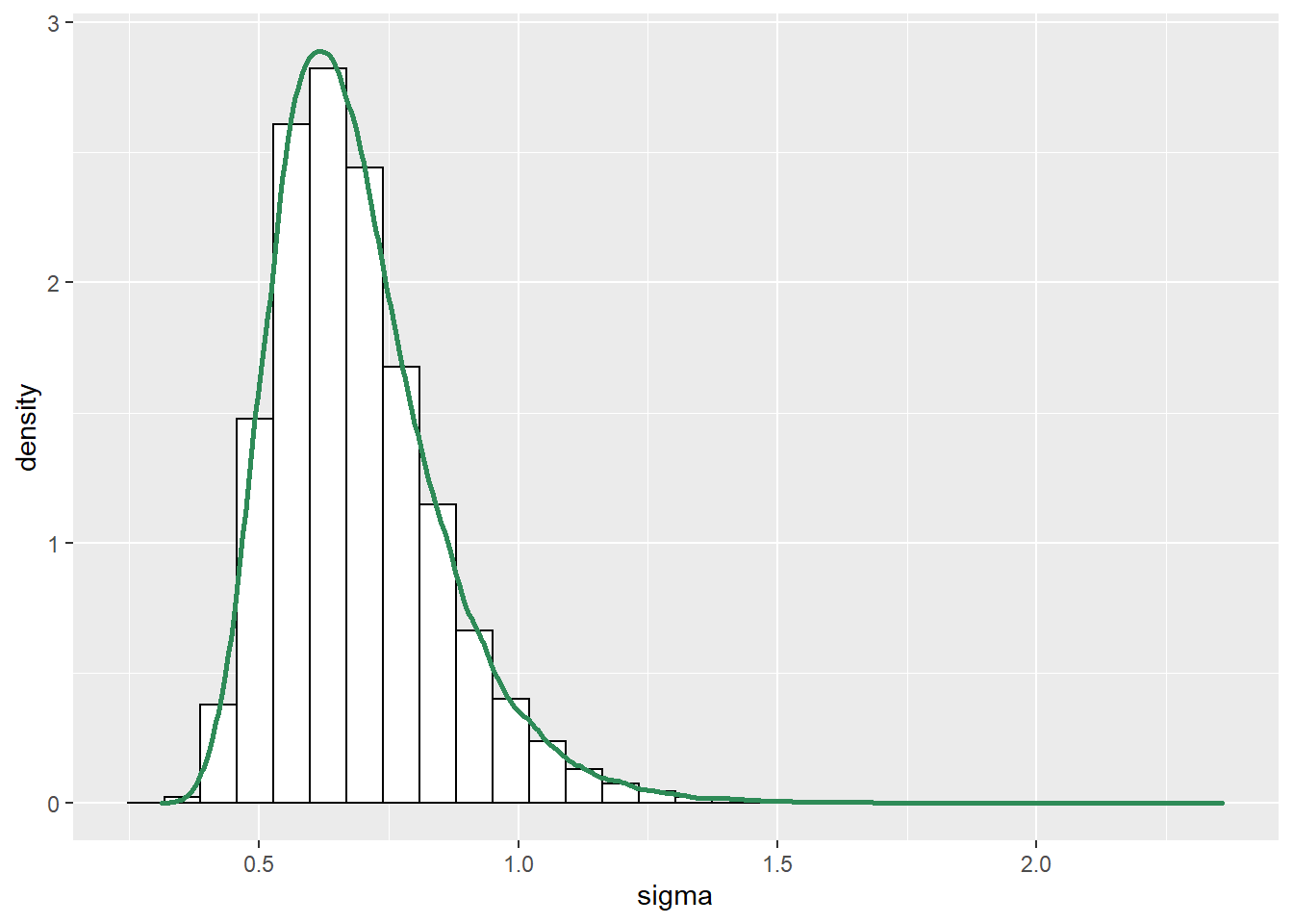
ggplot(posterior_sim, aes(sigma)) +
 geom_histogram(aes(y=..density..), color = "black", fill = "white") +
 geom_density(size = 1, color = "seagreen")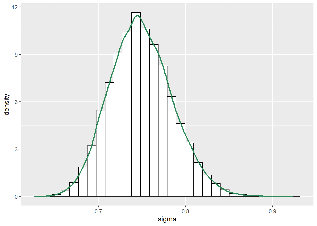
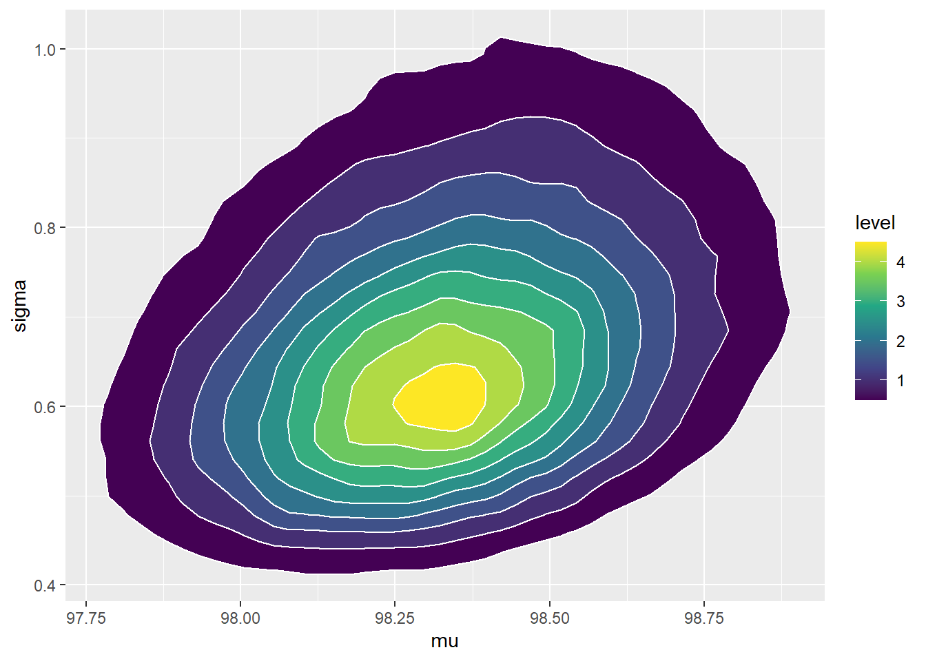
ggplot(posterior_sim, aes(mu, sigma)) +
  stat_density_2d(aes(fill = ..level..),
                  geom = "polygon", color = "white") +
     scale_fill_viridis_c()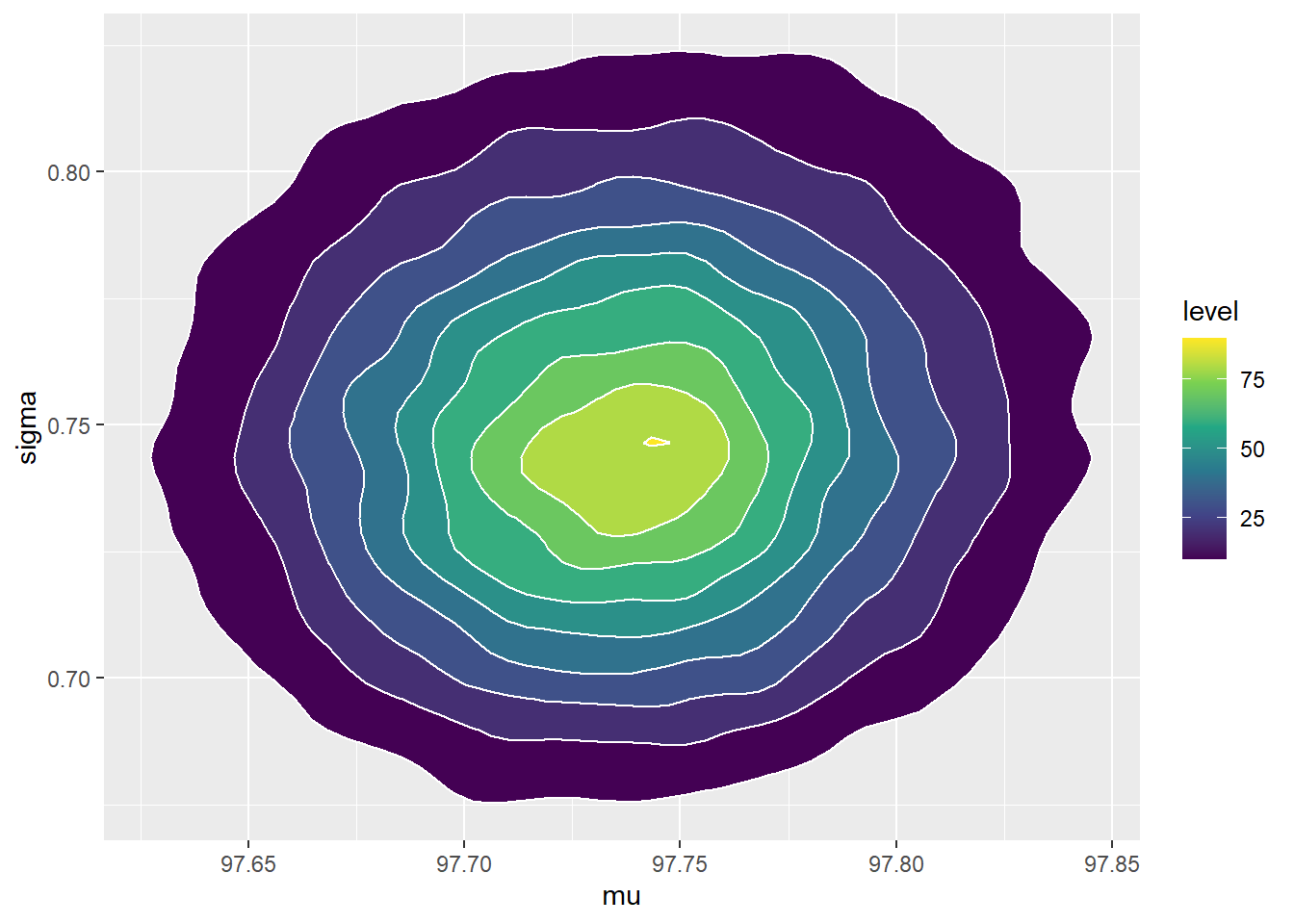
A few comments about the posterior distribution
- The joint posterior distribution appears to be roughly Bivariate Normal. The correlation is close to 0, indicating independence27 between \(\mu\) and \(\sigma\) in the posterior.
- The posterior distribution of \(\mu\) is approximately Normal with posterior mean 97.7 (basically the sample mean) and posterior SD 0.05. There is a 98% posterior probability that the population mean human body temperature is between 97.6 and 97.9 degrees F.
- The posterior distribution of \(\sigma\) is approximately Normal with posterior mean 0.75 (basically the sample SD) and posterior SD 0.036. There is a 98% posterior probability that the population SD of human body temperatures is between 0.67 and 0.84 degrees F.
- Since \(\mu\) and \(\sigma\) are roughly independent in the posterior, there is a posterior probability of 96% that both of the above statements are true, that is, that both parameters lie in their respective credible intervals. To have joint posterior credibility of 98%, we could lengthen each interval (to 99% for two independent intervals) to obtain a rectangular credibility region. The scatterplot also shows a 98% posterior credible ellipse (in black) for both \(\mu\) and \(\sigma\).
- Simulate a \((\mu, \sigma)\) pair from the joint posterior distribution.
- Given \(\mu\) and \(\sigma\), simulate a value of \(y\) from a \(N(\mu, \sigma)\) distribution.
- Repeat many times and summarize the simulated \(y\) values to approximate the posterior predictive distribution.
See the code below. JAGS has already returned a simulation from the joint posterior distribution of \((\mu, \sigma)\) For each of these simulated values, simulate a corresponding \(y\) value like usual.
theta_sim = as.matrix(posterior_sample)

y_sim = rnorm(nrow(theta_sim), theta_sim[, "mu"], theta_sim[, "sigma"])

hist(y_sim, freq = FALSE, xlab = "Body temperature (degrees F)",
     main = "Posterior preditive distribution")
lines(density(y_sim))
abline(v = quantile(y_sim, c(0.025, 0.975)), col = "orange")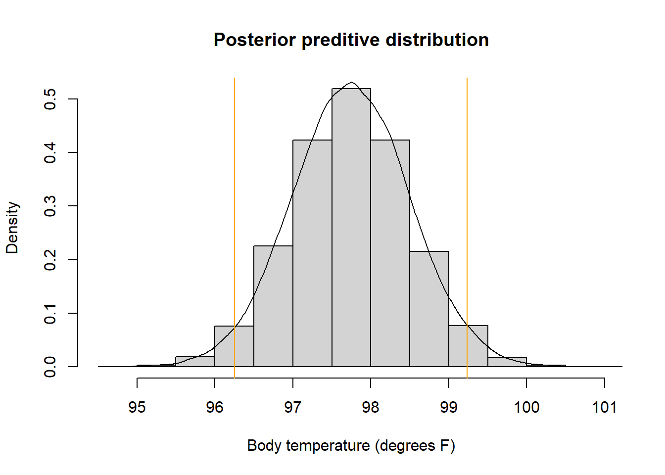
quantile(y_sim, c(0.025, 0.975))## 2.5% 97.5%
## 96.25 99.23There is a posterior predictive probability of 95% that a body temperature is between 96.25 and 99.20 degrees F. Roughly, 95% of healthy human body temperatures are between 96.25 and 99.20 degrees F.