Chapter 7 Introduction to Prediction

A Bayesian analysis leads directly and naturally to making predictions about future observations from the random process that generated the data. Prediction is also useful for checking if model assumptions seem reasonable in light of observed data.

Example 7.1 Do people prefer to use the word “data” as singular or plural? Data journalists at FiveThirtyEight conducted a poll to address this question (and others). Rather than simply ask whether the respondent considered “data” to be singular or plural, they asked which of the following sentences they prefer:

Some experts say it’s important to drink milk, but the data is inconclusive.
Some experts say it’s important to drink milk, but the data are inconclusive.

Suppose we wish to study the opinions of students in Cal Poly statistics classes regarding this issue. That is, let $\theta$ represent the population proportion of students in Cal Poly statistics classes who prefer to consider data as a singular noun, as in option a) above.

To illustrate ideas, we’ll start with a prior distribution which places probability 0.01, 0.05, 0.15, 0.30, 0.49 on the values 0.1, 0.3, 0.5, 0.7, 0.9, respectively.

Before observing any data, suppose we plan to randomly select a single Cal Poly statistics student. Consider the unconditional prior probability that the selected student prefers data as singular. (This is called a prior predictive probability.) Explain how you could use simulation to approximate this probability.
Compute the prior predictive probability from the previous part.
Before observing any data, suppose we plan to randomly select a sample of 35 Cal Poly statistics students. Consider the unconditional prior distribution of the number of students in the sample who prefer data as singular. (This is called a prior predictive distribution.) Explain how you could use simulation to approximate this distribution. In particular, how could you use simulation to approximate the prior predictive probability that at least 34 students in the sample prefer data as singular?
Compute and interpret the prior predictive probability that at least 34 students in a sample of size 35 prefer data as singular.

For the remaining parts, suppose that 31 students in a sample of 35 Cal Poly statistics students prefer data as singular.
Find the posterior distribution of $\theta$.
Now suppose we plan to randomly select an additional Cal Poly statistics student. Consider the posterior predictive probability that this student prefers data as singular. Explain how you could use simulation to estimate this probability.
Compute the posterior predictive probability from the previous part.
Suppose we plan to collect data on another sample of $35$ Cal Poly statistics students. Consider the posterior predictive distribution of the number of students in the new sample who prefer data as singular. Explain how you could use simulation to approximate this distribution. In particular, how could you use simulation to approximate the prior predictive probability that at least 34 students in the sample prefer data as singular? (Of course, the sample size of the new sample does not have to be 35. However, we’re keeping it the same so we can compare the prior and posterior predictions.)
Compute and interpret the posterior predictive probability that at least 34 students in a sample of size 35 prefer data as singular.

\iffalse{} Solution. to Example 7.1

If we knew what $\theta$ was, this probability would just be $\theta$. For example, if $\theta=0.9$, then there is a probability of 0.9 that a randomly selected student prefers data singular. If $\theta$ were 0.9, we could approximate the probability by constructing a spinner with 90% of the area marked as “success”, spinning it many times, and recording the proportion of spins that land on success, which should be roughly 90%. However, 0.9 is only one possible value of $\theta$. Since we don’t know what $\theta$ is, we need to first simulate a value of it, giving more weight to $\theta$ values with high prior probability. Therefore, we
1. Simulate a value of $\theta$ from the prior distribution.
2. Given the value of $\theta$, construct a spinner that lands on success with probability $\theta$. Spin the spinner once and record the result, success or not.
3. Repeat steps 1 and 2 many times, and find the proportion of repetitions which result in success. This proportion approximates the unconditional prior probability of success.
Use the law of total probability, where the weights are given by the prior probabilities. \[ 0.1(0.01) + 0.3(0.05) + 0.5(0.15) + 0.7(0.30) + 0.9(0.49) = 0.742 \] (This calculation is equivalent to the expected value of $\theta$ according to its prior distributon, that is, the prior mean.)
If we knew what $\theta$ was, we could construct a spinner than lands on success with probability $\theta$, spin it 35 times, and count the number of successes. Since we don’t know what $\theta$ is, we need to first simulate a value of it, giving more weight to $\theta$ values with high prior probability. Therefore, we
1. Simulate a value of $\theta$ from the prior distribution.
2. Given the value of $\theta$, construct a spinner that lands on success with probability $\theta$. Spin the spinner 35 times and count $y$, the number of spins that land on success.
3. Repeat steps 1 and 2 many times, and record the number of successes (out of 35) for each repetition. Summarize the simulated $y$ values to approximate the prior predictive distribution. To approximate the prior predictive probability that at least 34 students in a sample of size 35 prefer data as singular, count the number of simulated repetitions that result in at least 34 successes ($y \ge 34$) and divide by the total number of simulated repetitions.
If we knew $\theta$, the probability of at least 34 (out of 35) successes is, from a Binomial distribution, \[ 35\theta^{34}(1-\theta) + \theta^{35} \] Use the law of total probability again. \[\begin{align*} & \left(35(0.1)^{34}(1-0.1) + 0.1^{35}\right)(0.01) + \left(35(0.3)^{34}(1-0.3) + 0.3^{35}\right)(0.05)\\ & + \left(35(0.5)^{34}(1-0.5) + 0.5^{35}\right)(0.15) + \left(35(0.7)^{34}(1-0.7) + 0.7^{35}\right)(0.30)\\ & + \left(35(0.9)^{34}(1-0.9) + 0.9^{35}\right)(0.49) = 0.06 \end{align*}\]

According to this model, about 6% of samples of size 35 would result in at least 34 successes. The value 0.06 accounts for both (1) our prior uncertainty about $\theta$, (2) sample-to-sample variability in the number of successes $y$.

The likelihood is $\binom{35}{31}\theta^{31}(1-\theta)^{4}$, a function of $\theta$; dbinom(31, 35, theta). The posterior places almost all probability on $\theta = 0.9$, due to both its high prior probability and high likelihood.

theta = seq(0.1, 0.9, 0.2)

# prior
prior = c(0.01, 0.05, 0.15, 0.30, 0.49)

# data
n = 35 # sample size
y = 31 # sample count of success

# likelihood, using binomial
likelihood = dbinom(y, n, theta) # function of theta

# posterior
product = likelihood * prior
posterior = product / sum(product)

# bayes table
bayes_table = data.frame(theta,
                     prior,
                     likelihood,
                     product,
                     posterior)

bayes_table %>%
  adorn_totals("row") %>%
  kable(digits = 4, align = 'r')

theta	prior	likelihood	product	posterior
0.1	0.01	0.0000	0.0000	0.0000
0.3	0.05	0.0000	0.0000	0.0000
0.5	0.15	0.0000	0.0000	0.0000
0.7	0.30	0.0067	0.0020	0.0201
0.9	0.49	0.1998	0.0979	0.9799
Total	1.00	0.2065	0.0999	1.0000

The simulation would be similar to the prior simulation, but now we simulate $\theta$ from its posterior distribution rather than the prior distribution.
1. Simulate a value of $\theta$ from the posterior distribution.
2. Given the value of $\theta$, construct a spinner that lands on success with probability $\theta$. Spin the spinner once and record the result, success or not.
3. Repeat steps 1 and 2 many times, and find the proportion of repetitions which result in success. This proportion approximates the unconditional posterior probability of success.
Use the law of total probability, where the weights are given by the posterior probabilities. \[ 0.1(0.0000) + 0.3(0.0000) + 0.5(0.0000) + 0.7(0.0201) + 0.9(0.9799) = 0.8960 \] (This calculation is equivalent to the expected value of $\theta$ according to its posterior distributon, that is, the posterior mean.)
The simulation would be similar to the prior simulation, but now we simulate $\theta$ from its posterior distribution rather than the prior distribution.
1. Simulate a value of $\theta$ from the posterior distribution.
2. Given the value of $\theta$, construct a spinner that lands on success with probability $\theta$. Spin the spinner 35 times and count the number of spins that land on success.
3. Repeat steps 1 and 2 many times, and record the number of successes (out of 35) for each repetition. Summarize the simulated values to approximate the posterior predictive distribution. To approximate the posterior predictive probability that at least 34 students in a sample of size 35 prefer data as singular, count the number of simulated repetitions that result in at least 34 successes and divide by the total number of simulated repetitions.
Since the posterior probability that $\theta$ equals 0.9 is close to 1, the posterior predictive distribution would be close to, but not quite, the Binomial(35, 0.9) distribution.
Use the law of total probability again, but with the posterior probabilities rather than the prior probabilities as the weights. \[\begin{align*} & \left(35(0.1)^{34}(1-0.1) + 0.1^{35}\right)(0.0000) + \left(35(0.3)^{34}(1-0.3) + 0.3^{35}\right)(0.0000)\\ & + \left(35(0.5)^{34}(1-0.5) + 0.5^{35}\right)(0.0000) + \left(35(0.7)^{34}(1-0.7) + 0.7^{35}\right)(0.0201)\\ & + \left(35(0.9)^{34}(1-0.9) + 0.9^{35}\right)(0.9799) = 0.1199 \end{align*}\] According to this posterior model, about 12% of samples of size 35 would result in at least 34 successes. The value 0.12 accounts for both (1) our posterior uncertainty about $\theta$, after observing the sample data, (2) sample-to-sample variability in the number of successes $y$ for the yet-to-be-observed sample.

The plots below illustrate the distributions from the previous example.

The first plot below illustrates the conditional distribution of $Y$ given each value of $\theta$.

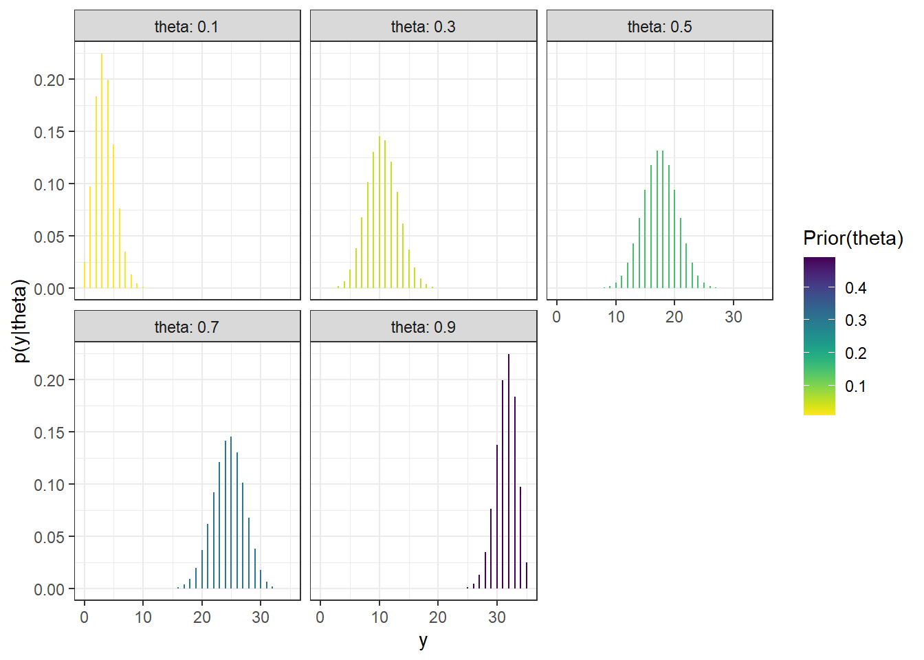
$Sample-to-sample distribution of $Y$, the number of successes in samples of size $n=35$ for different values of $\theta$ in Example 7.1. Color represents the prior probability of $\theta$, with darker colors corresponding to higher prior probability.$

Figure 7.1: Sample-to-sample distribution of $Y$, the number of successes in samples of size $n=35$ for different values of $\theta$ in Example 7.1. Color represents the prior probability of $\theta$, with darker colors corresponding to higher prior probability.

In the plot above, the prior distribution of $\theta$ is represented by color. The prior predictive distribution of $Y$ mixes the five conditional distributions in the previous plot, weighting by the prior distribution of $\theta$, to obtain the unconditional prior predictive distribution of $Y$.

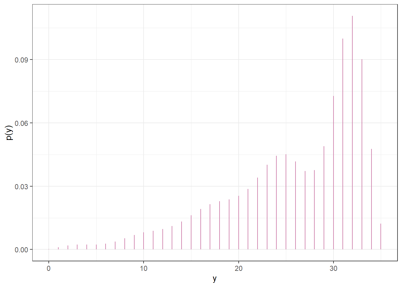
$Prior predictive distribution of $Y$, the number of successes in samples of size $n=35$, in Example 7.1.$

Figure 7.2: Prior predictive distribution of $Y$, the number of successes in samples of size $n=35$, in Example 7.1.

The prior predictive distribution reflects the sample-to-sample variability of the number of successes over many samples of size $n=35$, accounting for the prior uncertainty of $\theta$.

After observing a sample, we compute the posterior distribution of $\theta$ as usual. The following plot is similar to Figure 7.1, with the colors revised to reflect the posterior probabilities of the values of $\theta$.

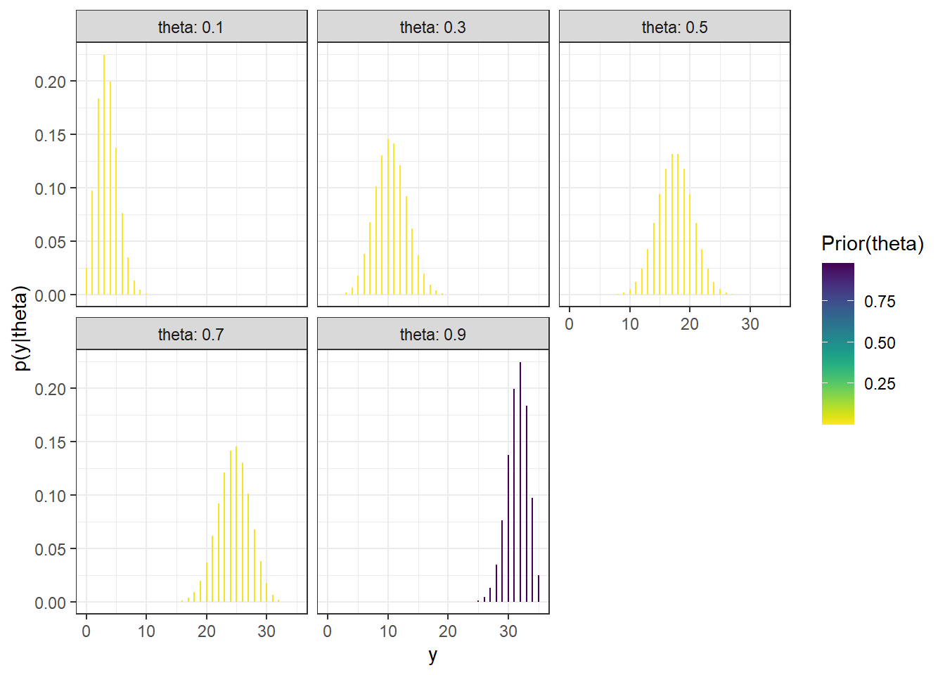
$Sample-to-sample distribution of $Y$, the number of successes in samples of size $n=35$ for different values of $\theta$ in Example 7.1. Color represents the posterior probability of $\theta$, after observing data from a different sample of size 35, with darker colors corresponding to higher posterior probability.$

Figure 7.3: Sample-to-sample distribution of $Y$, the number of successes in samples of size $n=35$ for different values of $\theta$ in Example 7.1. Color represents the posterior probability of $\theta$, after observing data from a different sample of size 35, with darker colors corresponding to higher posterior probability.

The posterior predictive distribution of $Y$ mixes the five conditional distributions in the previous plot, weighting by the posterior distribution of $\theta$, to obtain the unconditional posterior predictive distribution of $Y$. Since the posterior distribution of $\theta$ places almost all posterior probability on the value 0.9, the posterior predictive distribution of $Y$ is very similar to the conditional distribution of $Y$ given $\theta = 0.9$.

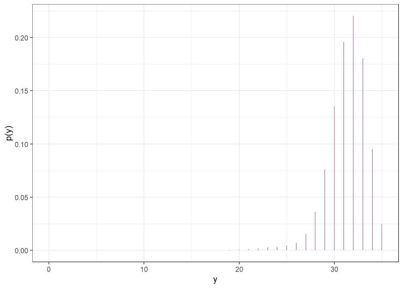
$Posterior predictive distribution of $Y$, the number of successes in samples of size $n=35$, in Example 7.1 after observing data from a different sample of size 35.$

Figure 7.4: Posterior predictive distribution of $Y$, the number of successes in samples of size $n=35$, in Example 7.1 after observing data from a different sample of size 35.

The predictive distribution of a random variable is the marginal distribution (of the unobserved values) after accounting for the uncertainty in the parameters. A prior predictive distribution is calculated using the prior distribution of the parameters. A posterior predictive distribution is calculated using the posterior distribution of the parameters, conditional on the observed data.

Be sure to carefully distinguish between posterior distributions and posterior predictive distributions (or between prior distributions and prior predictive distributions.)

Prior and posterior distributions are distributions on values of the parameters. These distributions quantify the degree of uncertainty about the unknown parameter $\theta$ (before and after observing data).

On the other hand, prior and posterior predictive distributions are distribution on potential values of the data. Predictive distributions reflect sample-to-sample variability of the sample data, while accounting for the uncertainty in the parameters.

Predictive probabilities can be computed via the law of total probability, as weighted averages over possible values of $\theta$. However, even when conditional distributions of data given the parameters are well known (e.g., Binomial($n$, $\theta$)), marginal distributions of the data are often not. Simulation is an effective tool in approximating predictive distributions.

Step 1: Simulate a value of $\theta$ from its posterior distribution (or prior distribution).
Step 2: Given this value of $\theta$ simulate a value of $y$ from $f(y|\theta)$, the data model conditional on $\theta$.
Repeat many times to simulate many $(\theta, y)$ pairs, and summarize the values of $y$ to approximate the posterior predictive distribution (or prior predictive distribution).

Example 7.2 Continuing the previous example. We’ll use a grid approximation and assume that any multiple of 0.0001 is a possible value of $\theta$: $0, 0.0001, 0.0002, \ldots, 0.9999, 1$.

Consider the context of this problem and sketch your prior distribution for $\theta$. What are the main features of your prior?
Assume the prior distribution for $\theta$ is proportional to $\theta^2$. Plot this prior distribution and describe its main features.
Given the shape of the prior distribution, explain why we might not want to compute central prior credible intervals. Suggest an alternative approach, and compute and interpret 50%, 80%, and 98% prior credible intervals for $\theta$.
Before observing any data, suppose we plan to randomly select a sample of 35 Cal Poly statistics students. Let $Y$ represent the number of students in the selected sample who prefer data as singular. Use simulation to approximate the prior predictive distribution of $Y$ and plot it.
Use software to compute the prior predictive distribution of $Y$. Compare to the simulation results.
Find a 95% prior prediction interval for $Y$. Write a clearly worded sentence interpreting this interval in context.

For the remaining parts, suppose that 31 students in a sample of 35 Cal Poly statistics students prefer data as singular.
Use software to plot the prior distribution and the (scaled) likelihood, then find the posterior distribution of $\theta$ and plot it and describe its main features.
Find and interpret 50%, 80%, and 98% central posterior credible intervals for $\theta$.
Suppose we plan to randomly select another sample of 35 Cal Poly statistics students. Let $\tilde{Y}$ represent the number of students in the selected sample who prefer data as singular. Use simulation to approximate the posterior predictive distribution of $\tilde{Y}$ and plot it. (Of course, the sample size of the new sample does not have to be 35. However, we’re keeping it the same so we can compare the prior and posterior predictions.)
Use software to compute the posterior predictive distribution of $\tilde{Y}$. Compare to the simulation results.
Find a 95% posterior prediction interval for $\tilde{Y}$. Write a clearly worded sentence interpreting this interval in context.
Now suppose instead of using the Cal Poly sample data (31/35) to form the posterior distribution of $\theta$, we had used the data from the FiveThirtyEight study in which 865 out of 1093 respondents preferred data as singular. Use software to plot the prior distribution and the (scaled) likelihood, then find the posterior distribution of $\theta$ and plot it and describe its main features. In particular, find and interpret a 98% central posterior credible interval for $\theta$. How does the posterior based on the FiveThirtyEight data compare to the posterior distribution based on the Cal Poly sample data (31/35)? Why?
Again, suppose we use the FiveThirtyEight data to form the posterior distribution of $\theta$. Suppose we plan to randomly select a sample of 35 Cal Poly statistics students. Let $\tilde{Y}$ represent the number of students in the selected sample who prefer data as singular. Use simulation to approximate the posterior predictive distribution of $\tilde{Y}$ and plot it. In particular, find and interpret a 95% posterior prediction interval for $\tilde{Y}$. How does the predictive distribution which uses the posterior distribution based on the FiveThirtyEight data compare to the one based on the Cal Poly sample data (31/35)? Why?

\iffalse{} Solution. to Example 7.2

Results will of course vary, but do consider what your prior would look like.

We believe a majority, and probably a strong majority, of students will prefer data as singular. The prior mode is 1, the prior mean is 0.75, and the prior standard deviation is 0.19.

theta = seq(0, 1, 0.0001)

# prior
prior = theta ^ 2
prior = prior / sum(prior)

ylim = c(0, max(prior))
plot(theta, prior, type='l', xlim=c(0, 1), ylim=ylim, col="skyblue", xlab='theta', ylab='')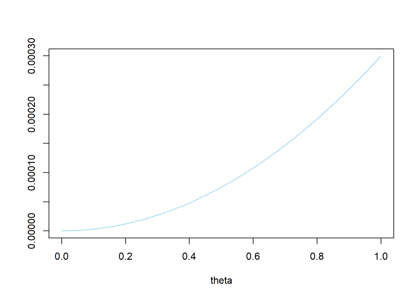

# prior mean
prior_ev = sum(theta * prior)
prior_ev

## [1] 0.75

# prior variance
prior_var = sum(theta ^ 2 * prior) - prior_ev ^ 2

# prior sd
sqrt(prior_var)

## [1] 0.1937

Central credibles would exclude $\theta$ values near 1, but these are the values with highest prior probability. For example, a central 50% prior credible interval is [0.630, 0.909], but this excludes values of $\theta$ with the highest prior probability. An alternative is to use highest prior probability intervals. For this prior, it seems reasonable to just fix the upper endpoint of the credible intervals to be 1, and to find the lower endpoint corresponding to the desired probability. The lower bound of such a 50% credible interval is the 50th percentile; of an 80% credible interval is the 20th percentile; of a 98% credible interval is the 2nd percentile. There is a prior probability of 50% that at least 79.4% of Cal Poly students prefer data as singular; it’s equally plausible that $\theta$ is above 0.794 as below.
There is a prior probability of 80% that at least 58.5% of Cal Poly students prefer data as singular; it’s four times more plausible that $\theta$ is above 0.585 than below. There is a prior probability of 98% that at least 27.1% of Cal Poly students prefer data as singular; it’s 49 times more plausible that $\theta$ is above 0.271 than below.
```
prior_cdf = cumsum(prior)

# 50th percentile
theta[max(which(prior_cdf <= 0.5))]
```
```
## [1] 0.7936
```
```
# 10th percentile
theta[max(which(prior_cdf <= 0.2))]
```
```
## [1] 0.5847
```
```
# 2nd percentile
theta[max(which(prior_cdf <= 0.02))]
```
```
## [1] 0.2714
```
We use the sample function with the prob argument to simulate a value of $\theta$ from its prior distribution, and then use rbinom to simulate a sample. The table below displays the results of a few repetitions of the simulation.
```
n = 35

n_sim = 10000

theta_sim = sample(theta, n_sim, replace = TRUE, prob = prior)

y_sim = rbinom(n_sim, n, theta_sim)

data.frame(theta_sim, y_sim) %>%
  head(10) %>%
  kable(digits = 5)
```
theta_sim y_sim

0.6711 26

0.7621 26

0.8947 33

0.8719 30

0.5030 16

0.9272 34

0.8771 31

0.6362 25

0.8140 29

0.1598 3

theta_sim	y_sim
0.6711	26
0.7621	26
0.8947	33
0.8719	30
0.5030	16
0.9272	34
0.8771	31
0.6362	25
0.8140	29
0.1598	3

We program the law of total probability calculation for each possible value of $y$. (There are better ways of doing this than a for loop, but it’s good enough.)

# Predictive distribution
y_predict = 0:n

py_predict = rep(NA, length(y_predict))

for (i in 1:length(y_predict)) {
  py_predict[i] = sum(dbinom(y_predict[i], n, theta) * prior) # prior
}

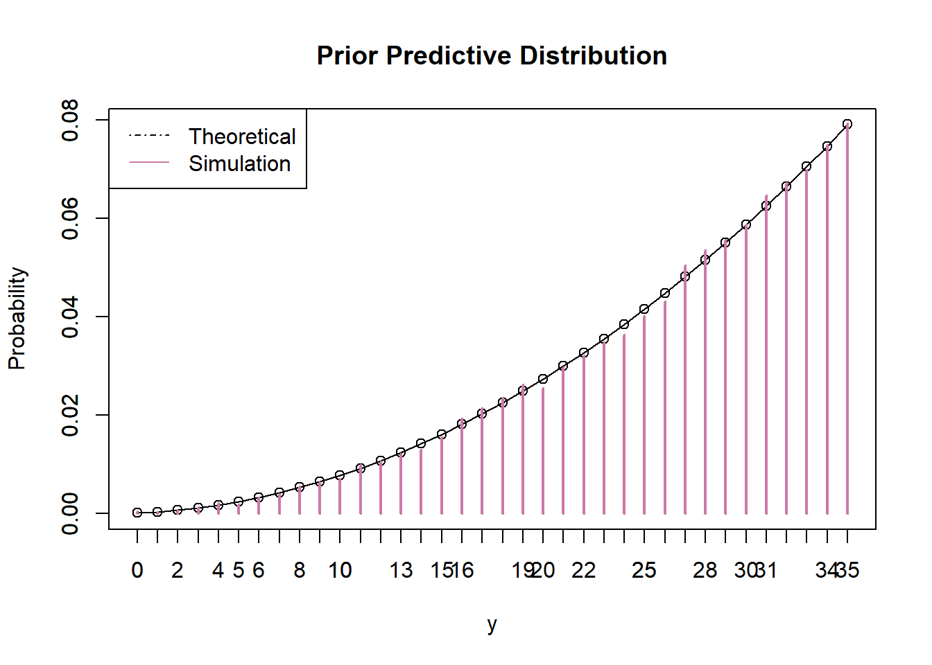
# Prediction interval
py_predict_cdf = cumsum(py_predict)
c(y_predict[max(which(py_predict_cdf <= 0.025))], y_predict[min(which(py_predict_cdf >= 0.975))])

## [1]  8 35

There is prior predictive probability of 95% that between 8 and 35 students in a sample of 35 students will prefer data as singular.

For the remaining parts, suppose that 31 students in a sample of 35 Cal Poly statistics students prefer data as singular.

The observed sample proportion is 31/35=0.886. The posterior distribution is slightly skewed to the left with a posterior mean of 0.872 and a posterior standard deviation of 0.053.

# data
n = 35 # sample size
y = 31 # sample count of success

# likelihood, using binomial
likelihood = dbinom(y, n, theta) # function of theta

# posterior
product = likelihood * prior
posterior = product / sum(product)

# posterior mean
posterior_ev = sum(theta * posterior)
posterior_ev

## [1] 0.8718

# posterior variance
posterior_var = sum(theta ^ 2 * posterior) - posterior_ev ^ 2

# posterior sd
sqrt(posterior_var)

## [1] 0.05286

# posterior cdf
posterior_cdf = cumsum(posterior)

# posterior 50% central credible interval
c(theta[max(which(posterior_cdf <= 0.25))], theta[min(which(posterior_cdf >= 0.75))])

## [1] 0.8397 0.9106

# posterior 80% central credible interval
c(theta[max(which(posterior_cdf <= 0.1))], theta[min(which(posterior_cdf >= 0.9))])

## [1] 0.8005 0.9346

# posterior 98% central credible interval
c(theta[max(which(posterior_cdf <= 0.01))], theta[min(which(posterior_cdf >= 0.99))])

## [1] 0.7238 0.9651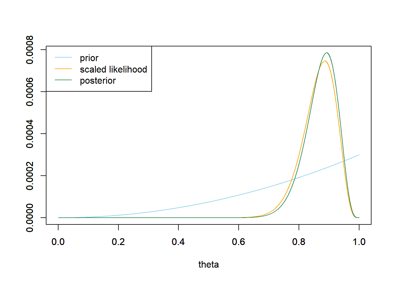

There is a posterior probability of 50% that between 84.0% and 91.1% of Cal Poly students prefer data as singular; after observing the sample data, it’s equally plausible that $\theta$ is inside [0.840, 0.911] as outside. There is a posterior probability of 80% that between 80.0% and 93.5% of Cal Poly students prefer data as singular; after observing the sample data, it’s four times mores plausible that $\theta$ is inside [0.800, 0.935] as outside. There is a posterior probability of 98% that between 72.4% and 96.5% of Cal Poly students prefer data as singular; after observing the sample data, it’s 49 times mores plausible that $\theta$ is inside [0.724, 0.965] as outside.
Similar to the prior simulation, but now we simulate $\theta$ based on its posterior distribution. The table below displays the results of a few repetitions of the simulation.
```
theta_sim = sample(theta, n_sim, replace = TRUE, prob = posterior)

y_sim = rbinom(n_sim, n, theta_sim)

  data.frame(theta_sim, y_sim) %>%
  head(10) %>%
  kable(digits = 5)
```
theta_sim y_sim

0.8304 30

0.8823 32

0.9251 30

0.9442 35

0.9069 32

0.9083 32

0.9564 34

0.8123 32

0.7888 30

0.8705 29

theta_sim	y_sim
0.8304	30
0.8823	32
0.9251	30
0.9442	35
0.9069	32
0.9083	32
0.9564	34
0.8123	32
0.7888	30
0.8705	29

Similar to the prior calculation, but now we use the posterior probabilities as the weights in the law of total probability calculation.

# Predictive distribution
y_predict = 0:n

py_predict = rep(NA, length(y_predict))

for (i in 1:length(y_predict)) {
  py_predict[i] = sum(dbinom(y_predict[i], n, theta) * posterior) # posterior
}

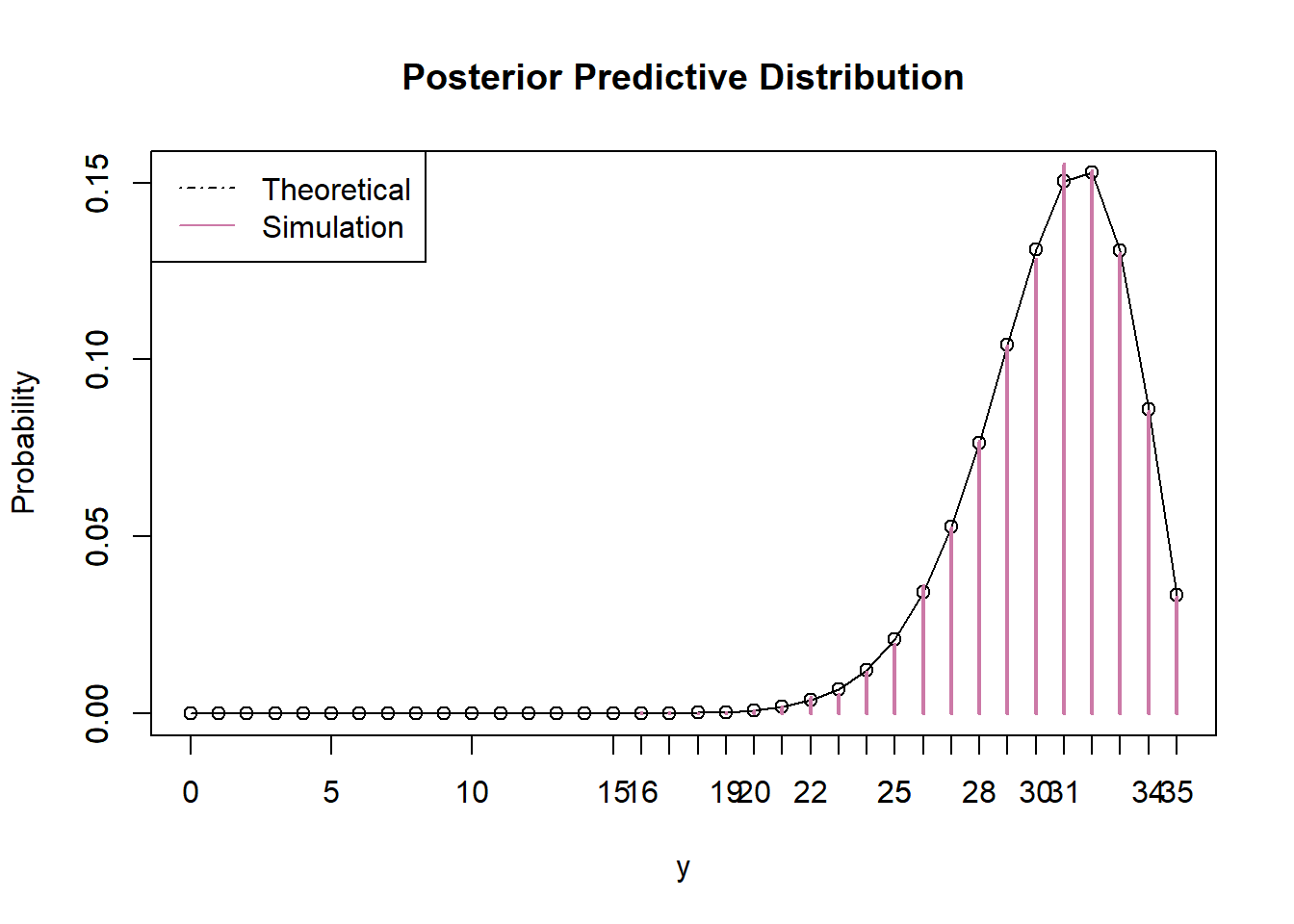
# Prediction interval
py_predict_cdf = cumsum(py_predict)
c(y_predict[max(which(py_predict_cdf <= 0.025))], y_predict[min(which(py_predict_cdf >= 0.975))])

## [1] 23 35

There is posterior predictive probability of 95% that between 23 and 35 students in a sample of 35 students will prefer data as singular.

The observed sample proportion is 865/1093=0.791. The posterior mean is 0.791, and the posterior standard deviation is 0.012. There is a posterior probability of 98% that between 76.2% and 81.9% of Cal Poly students prefer data as singular. The posterior SD is much smaller and the 98% credible interval is narrower based on the FiveThirtyEight due to the much larger sample size. (The posterior means and location of the credible intervals are also different due to the difference in sample proportions.)

# data
n = 1093 # sample size
y = 865 # sample count of success

# likelihood, using binomial
likelihood = dbinom(y, n, theta) # function of theta

# posterior
product = likelihood * prior
posterior = product / sum(product)

# posterior mean
posterior_ev = sum(theta * posterior)
posterior_ev

## [1] 0.7912

# posterior variance
posterior_var = sum(theta ^ 2 * posterior) - posterior_ev ^ 2

# posterior sd
sqrt(posterior_var)

## [1] 0.01227

# posterior 98% credible interval
posterior_cdf = cumsum(posterior)
c(theta[max(which(posterior_cdf <= 0.01))], theta[min(which(posterior_cdf >= 0.99))])

## [1] 0.7619 0.8190

There is posterior predictive probability of 95% that between 23 and 35 students in a sample of 35 students will prefer data as singular. Despite the fact that the posterior distributions of $\theta$ are different in the two scenarios, the posterior predictive distributions are fairly similar. Even though there is less uncertainty about $\theta$ in the FiveThirtyEight case, the predictive distribution reflects the sample-to-sample variability of the number of students who prefer data as singular, which is mainly impacted by the size of the sample being “predicted”. The table below displays a few repetitions of the posterior predictive simulation. Notice that all the $\theta$ values are around 0.79 or so, but there is still sample-to-sample variability in the $Y$ values.
```
n = 35

# Predictive simulation
theta_sim = sample(theta, n_sim, replace = TRUE, prob = posterior)

y_sim = rbinom(n_sim, n, theta_sim)

  data.frame(theta_sim, y_sim) %>%
  head(10) %>%
  kable(digits = 5)
```
theta_sim y_sim

0.7979 32

0.7768 27

0.7559 26

0.8000 33

0.7844 28

0.7823 30

0.7811 25

0.7660 23

0.8057 32

0.7910 27
```
# Predictive distribution
y_predict = 0:n

py_predict = rep(NA, length(y_predict))

for (i in 1:length(y_predict)) {
  py_predict[i] = sum(dbinom(y_predict[i], n, theta) * posterior) # posterior
}

# Prediction interval
py_predict_cdf = cumsum(py_predict)
c(y_predict[max(which(py_predict_cdf <= 0.025))], y_predict[min(which(py_predict_cdf >= 0.975))])
```
```
## [1] 22 32
```

theta_sim	y_sim
0.7979	32
0.7768	27
0.7559	26
0.8000	33
0.7844	28
0.7823	30
0.7811	25
0.7660	23
0.8057	32
0.7910	27

Be sure to distinguish between a prior/posterior distribution and a prior/posterior predictive distribution.

A prior/posterior distribution is a distribution on potential values of the parameters $\theta$. These distributions quantify the degree of uncertainty about the unknown parameter $\theta$ (before and after observing data).
A prior/posterior predictive distribution is a distribution on potential values of the data $y$. Predictive distributions reflect sample-to-sample variability of the sample data, while accounting for the uncertainty in the parameters.

Even if parameters are essentially “known” — that is, even if the prior/posterior variance of parameters is small — there will still be sample-to-sample variability reflected in the predictive distribution of the data, mainly influenced by the size $n$ of the sample being “predicted”.