8.2 Continuous distributions for a population proportion
We have seen a few examples where we used Normal distributions as prior distributions for a population proportion \(\theta\). Normal distributions are commonly used as priors, but they do not allow for asymmetric prior distributions. We’ll now consider Beta distributions, a family of distributions that are commonly used as prior distributions for population proportions.
Example 8.1 Continuing Example 7.1 where \(\theta\) represents the population proportion of students in Cal Poly statistics classes who prefer to consider data as a singular noun.
- Assume a continuous prior distribution for \(\theta\) which is proportional to \(\theta^2,\; 0<\theta<1\). Sketch this distribution.
- The previous part implies that \(\pi(\theta)=c \theta^2,\; 0<\theta<1\), for an appropriate constant \(c\). Find \(c\).
- Compute the prior mean of \(\theta\).
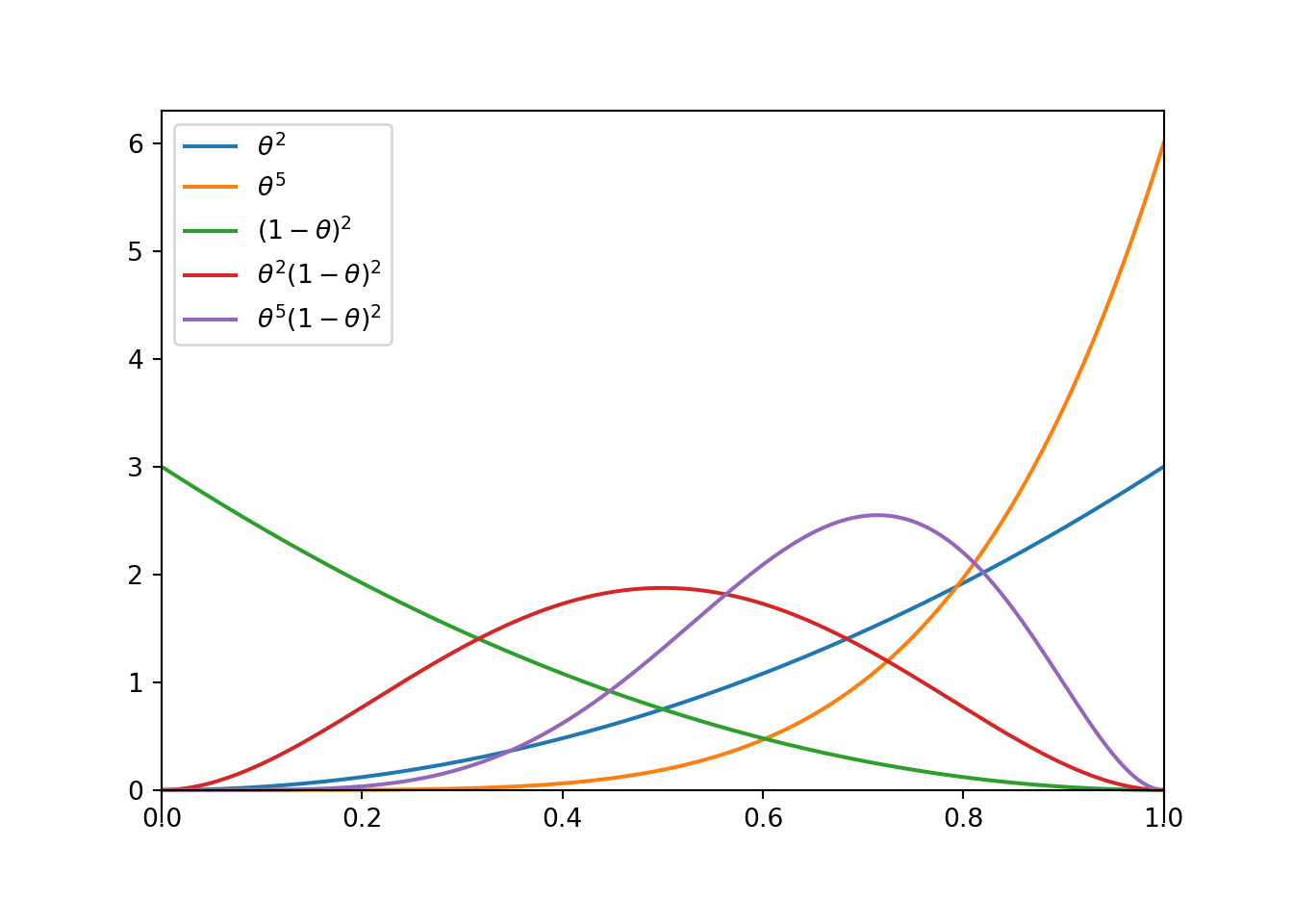
- Now we’ll consider a few more prior distributions. Sketch each of the following priors. How do they compare?
- proportional to \(\theta^2,\; 0<\theta<1\). (from previous)
- proportional to \(\theta^5,\; 0<\theta<1\).
- proportional to \((1-\theta)^2,\; 0<\theta<1\).
- proportional to \(\theta^2(1-\theta)^2,\; 0<\theta<1\).
- proportional to \(\theta^5(1-\theta)^2,\; 0<\theta<1\).
- See the plot below. The distribution is similar to the discrete grid approximation in Example 7.2.
- Set the total area under the curve equal to 1 and solve for \(c=3\) \[ 1 = \int_0^1 c\theta^2 d\theta = c \int_0^1 \theta^2d\theta = c (1/3) \Rightarrow c = 3 \]
- Since \(\theta\) is continuous we use calculus \[ E(\theta) = \int_0^1 \theta \,\pi(\theta)d\theta = \int_0^1 \theta (3\theta^2)d\theta = 3/4 \]
- See the plot below. The prior proportional to \((1-\theta)^2\) is the mirror image of the prior proportional to \(\theta^2\), reflected about 0.5. As the exponent on \(\theta\) increases, more density is shifted towards 1. As the exponent on \(1-\theta\) increases, more density is shifted towards 0. When the exponents are the same, the density is symmetric about 0.5
A continuous random variable \(U\) has a Beta distribution with shape parameters \(\alpha>0\) and \(\beta>0\) if its density satisfies15 \[ f(u) \propto u^{\alpha-1}(1-u)^{\beta-1}, \quad 0<u<1, \] and \(f(u)=0\) otherwise.
- If \(\alpha = \beta\) the distribution is symmetric about 0.5
- If \(\alpha > \beta\) the distribution is skewed to the left (with greater density above 0.5 than below)
- If \(\alpha < \beta\) the distribution is skewed to the right (with greater density below 0.5 than above)
- If \(\alpha = 1\) and \(\beta = 1\), the Beta(1, 1) distribution is the Uniform distribution on (0, 1).
It can be shown that a Beta(\(\alpha\), \(\beta\)) density has \[\begin{align*} \text{Mean (EV):} & \quad \frac{\alpha}{\alpha+\beta}\\ \text{Variance:} & \quad \frac{\left(\frac{\alpha}{\alpha+\beta}\right)\left(1-\frac{\alpha}{\alpha+\beta}\right)}{\alpha+\beta+1} \\ \text{Mode:} & \quad \frac{\alpha -1}{\alpha+\beta-2}, \qquad \text{(if $\alpha>1$, $\beta\ge1$ or $\alpha\ge1$, $\beta>1$)} \end{align*}\]
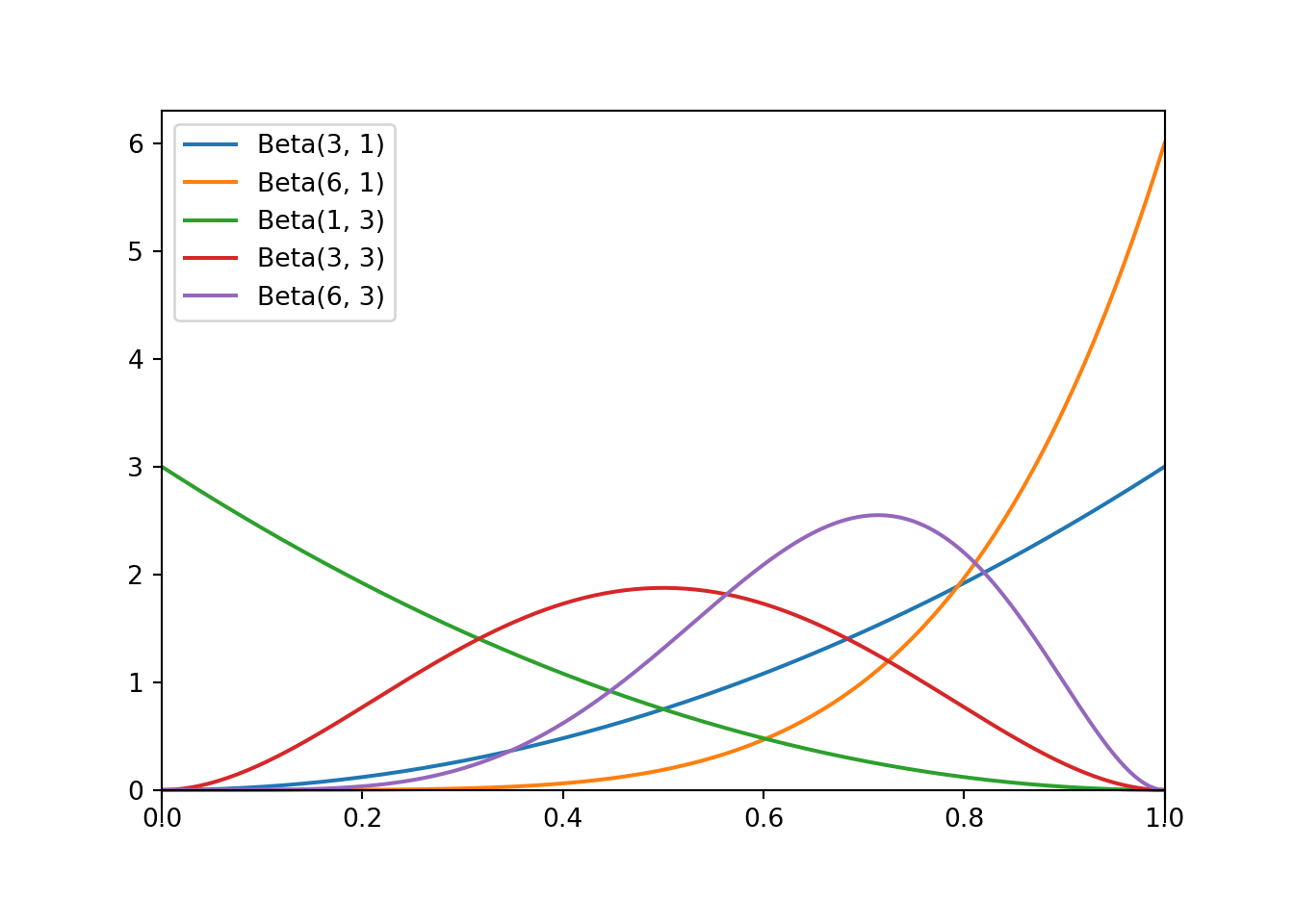
- Each of the previous distributions in the previous example was a Beta distribution. For each distribution, identify the shape parameters and the prior mean and standard deviation.
- proportional to \(\theta^2,\; 0<\theta<1\).
- proportional to \(\theta^5,\; 0<\theta<1\).
- proportional to \((1-\theta)^2,\; 0<\theta<1\).
- proportional to \(\theta^2(1-\theta)^2,\; 0<\theta<1\).
- proportional to \(\theta^5(1-\theta)^2,\; 0<\theta<1\).
- Now suppose that 31 students in a sample of 35 Cal Poly statistics students prefer data as singular. Specify the shape of the likelihood as a function of \(\theta, 0<\theta<1\).
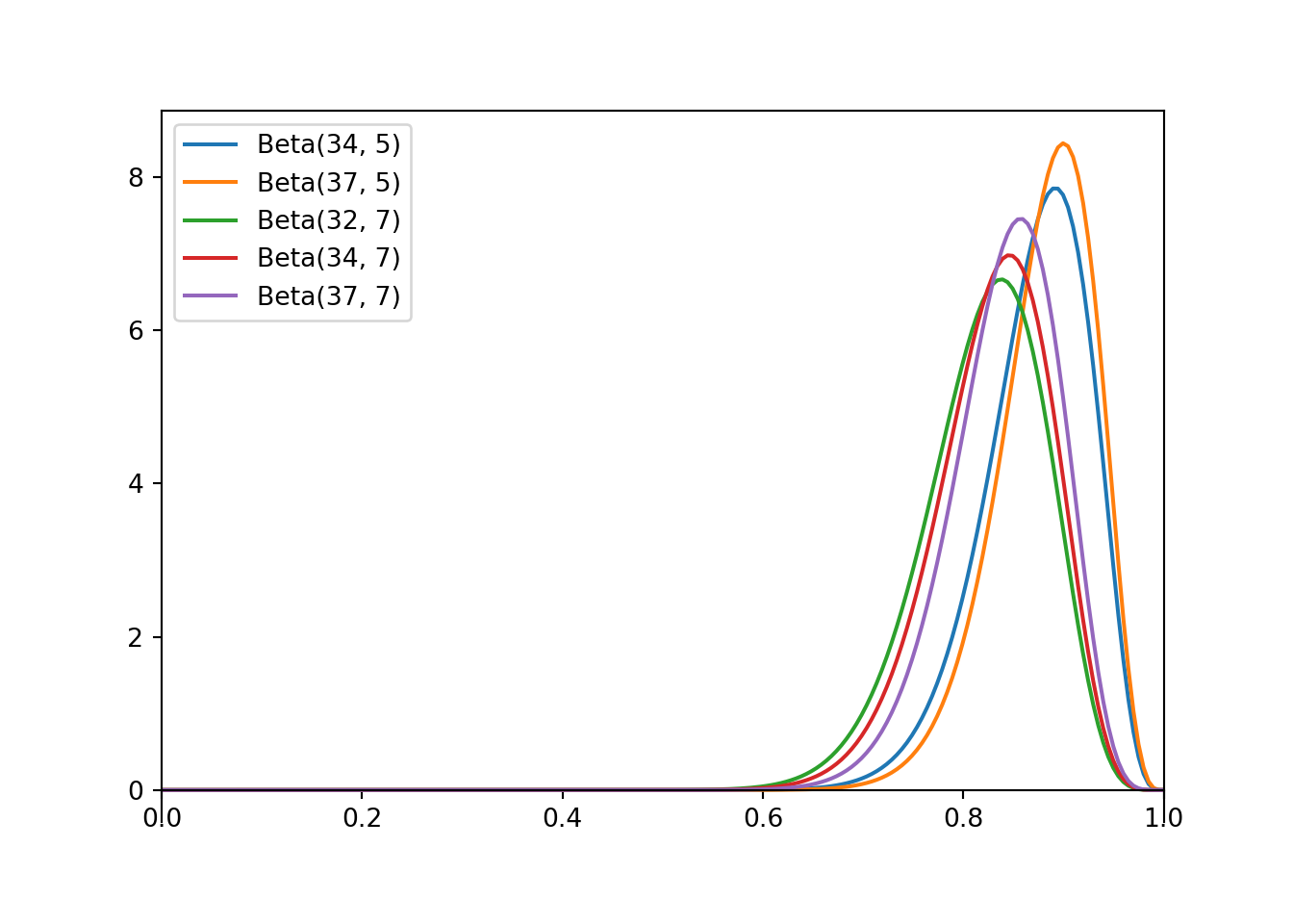
- Starting with each of the prior distributions from the first part, find the posterior distribution of \(\theta\) based on this sample, and identify it as a Beta distribution by specifying the shape parameters \(\alpha\) and \(\beta\)
- proportional to \(\theta^2,\; 0<\theta<1\).
- proportional to \(\theta^5,\; 0<\theta<1\).
- proportional to \((1-\theta)^2,\; 0<\theta<1\).
- proportional to \(\theta^2(1-\theta)^2,\; 0<\theta<1\).
- proportional to \(\theta^5(1-\theta)^2,\; 0<\theta<1\).
- For each of the posterior distributions in the previous part, compute the posterior mean and standard deviation. How does each posterior distribution compare to its respective prior distribution?
Careful with the exponents. For example, \(\theta^2 = \theta^2(1-\theta)^0 = \theta^{3-1}(1-\theta)^{1-1}\), which corresponds to a Beta(3, 1) distribution.
Distribution \(\alpha\) \(\beta\) Proportional to Mean SD a Beta(3, 1) 3 1 \(\theta^2, 0<\theta < 1\) 0.750 0.194 b Beta(6, 1) 6 1 \(\theta^5, 0<\theta < 1\) 0.857 0.124 c Beta(1, 3) 1 3 \((1-\theta)^2, 0<\theta < 1\) 0.250 0.194 d Beta(3, 3) 3 3 \(\theta^2(1-\theta)^2, 0<\theta < 1\) 0.500 0.189 e Beta(6, 3) 6 3 \(\theta^5(1-\theta)^2, 0<\theta < 1\) 0.667 0.149 Given \(\theta\), the number of students in the sample who prefer data as singular, \(Y\), follows a Binomial(35, \(\theta\)) distribution. The likelihood is the probability of observing \(Y=31\) viewed as a function of \(\theta\). \[\begin{align*} f(31|\theta) & = \binom{35}{31}\theta^{31}(1-\theta)^4, \qquad 0 < \theta <1\\ & \propto \theta^{31}(1-\theta)^4, \qquad 0 < \theta <1 \end{align*}\] The constant \(\binom{35}{31}\) does not affect the shape of the likelihood as a function of \(\theta\).
As always, the posterior distribution is proportional to the product of the prior distribution and the likelihood. For the Beta(3, 1) prior, the prior density is proportional to \(\theta^2\), \(0<\theta<1\), and for the observed data \(y=31\) with \(n=35\), the likelihood is proportional to \(\theta^{31}(1-\theta)^4\), \(0<\theta<1\). Therefore, the posterior density, as a function of \(\theta\), is proportional to \[\begin{align*} \pi(\theta|y = 31) & \propto \left(\theta^2\right)\left(\theta^{31}(1-\theta)^4\right), \qquad 0 <\theta < 1\\ & \propto \theta^{33}(1-\theta)^4, \qquad 0 <\theta < 1\\ & \propto \theta^{34 - 1}(1-\theta)^{5 - 1}, \qquad 0 <\theta < 1\\ \end{align*}\] Therefore, the posterior distribution of \(\theta\) is the Beta(3 + 31, 1 + 35 - 31), that is, the Beta(34, 5) distribution. The other situations are similar. The prior changes but the likelihood stays the same, based on a sample with 31 successes and \(35-31 = 4\) failures. If the prior distribution is Beta(\(\alpha\), \(\beta\)) then the posterior distribution is Beta(\(\alpha + 31\), \(\beta + 35 - 31\)).
Prior Distribution Posterior proportional to Posterior Distribution Posterior Mean Posterior SD a Beta(3, 1) \(\theta^{2 + 31}(1-\theta)^{0 + 4}, 0 < \theta < 1\) Beta(34, 5) 0.872 0.053 b Beta(6, 1) \(\theta^{5 + 31}(1-\theta)^{0 + 4}, 0 < \theta < 1\) Beta(37, 5) 0.881 0.049 c Beta(1, 3) \(\theta^{0 + 31}(1-\theta)^{2 + 4}, 0 < \theta < 1\) Beta(32, 7) 0.821 0.061 d Beta(3, 3) \(\theta^{2 + 31}(1-\theta)^{2 + 4}, 0 < \theta < 1\) Beta(34, 7) 0.829 0.058 e Beta(6, 3) \(\theta^{5 + 31}(1-\theta)^{2 + 4}, 0 < \theta < 1\) Beta(37, 7) 0.841 0.055 See the table above. Each posterior distribution concentrates more probability towards the observed sample proportion \(31/35 = 0.886\), though there are some small differences due to the prior. The posterior SD is less than the prior SD; there is less uncertainty about \(\theta\) after observing some data.
Beta distributions are often used in Bayesian models involving population proportions. Consider some binary (“success/failure”) variable and let \(\theta\) be the population proportion of success. Select a random sample of size \(n\) from the population and let \(Y\) count the number of successes in the sample.
Beta-Binomial model. If \(\theta\) has a Beta\((\alpha, \beta)\) prior distribution and the conditional distribution of \(Y\) given \(\theta\) is the Binomial\((n, \theta)\) distribution, then the posterior distribution of \(\theta\) given \(y\) is the Beta\((\alpha + y, \beta + n - y)\) distribution. \[\begin{align*} \text{prior:} & & \pi(\theta) & \propto \theta^{\alpha-1}(1-\theta)^{\beta-1}, \quad 0<\theta<1,\\ \\ \text{likelihood:} & & f(y|\theta) & \propto \theta^y (1-\theta)^{n-y}, \quad 0 < \theta < 1,\\ \\ \text{posterior:} & & \pi(\theta|y) & \propto \theta^{\alpha+y-1}(1-\theta)^{\beta+n-y-1}, \quad 0<\theta<1. \end{align*}\]
Try this applet which illustrates the Beta-Binomial model.
In a sense, you can interpret \(\alpha\) as “prior successes” and \(\beta\) as “prior failures”, but these are only “pseudo-observations”. Also, \(\alpha\) and \(\beta\) are not necessarily integers.
| Prior | Data | Posterior | |
|---|---|---|---|
| Successes | \(\alpha\) | \(y\) | \(\alpha + y\) |
| Failures | \(\beta\) | \(n-y\) | \(\beta + n - y\) |
| Total | \(\alpha+\beta\) | \(n\) | \(\alpha + \beta + n\) |
When the prior and posterior distribution belong to the same family, that family is called a conjugate prior distribution for the likelihood. So, the Beta distributions form a conjugate prior family for Binomial distributions.
Example 8.3 In Example 7.2 we used a grid approximation to the prior distribution of \(\theta\). Now we will assume a continuous prior distributions. Assume that \(\theta\) has a Beta(3, 1) prior distribution and that 31 students in a sample of 35 Cal Poly statistics students prefer data as singular.
- Plot the prior distribution, (scaled) likelihood, and posterior distribution.
- Use software to find 50%, 80%, and 98% central posterior credible intervals.
- Compare the results to those using the grid approximation in Example 7.2.
- Express the posterior mean as a weighted average of the prior mean and sample proportion. Describe what the weights are, and explain why they make sense.
See plot below. The posterior distribution is the Beta(34, 5) distribution. Note that the grid in the code is just to plot things in R. In particular, the posterior is computed using the Beta-Binomial model, not the grid.
theta = seq(0, 1, 0.0001) # the grid is just for plotting

# prior
alpha_prior = 3
beta_prior = 1
prior = dbeta(theta, alpha_prior, beta_prior)

# data
n = 35
y = 31

# likelihood
likelihood = dbinom(y, n, theta)

# posterior
alpha_post = alpha_prior + y
beta_post = beta_prior + n - y
posterior = dbeta(theta, alpha_post, beta_post)

# plot
ymax = max(c(prior, posterior))
scaled_likelihood = likelihood * ymax / max(likelihood)

plot(theta, prior, type='l', col='skyblue', xlim=c(0, 1), ylim=c(0, ymax), ylab='', yaxt='n')
par(new=T)
plot(theta, scaled_likelihood, type='l', col='orange', xlim=c(0, 1), ylim=c(0, ymax), ylab='',  yaxt='n')
par(new=T)
plot(theta, posterior, type='l', col='seagreen', xlim=c(0, 1), ylim=c(0, ymax), ylab='', yaxt='n')
legend("topleft", c("prior", "scaled likelihood", "posterior"), lty=1, col=c("skyblue", "orange", "seagreen"))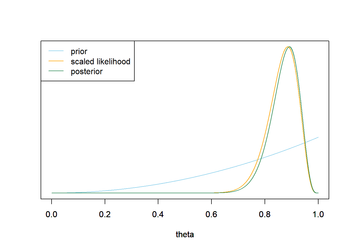
# 50% posterior credible interval
qbeta(c(0.25, 0.75), alpha_post, beta_post)
## [1] 0.8398 0.9106# 80% posterior credible interval qbeta(c(0.1, 0.9), alpha_post, beta_post)## [1] 0.8006 0.9346# 98% posterior credible interval qbeta(c(0.01, 0.99), alpha_post, beta_post)## [1] 0.7239 0.9651We can use
qbetato compute quantiles (a.k.a. percentiles). The posterior mean is 0.872, and the prior standard deviation is 0.053. There is a posterior probability of 50% that between 84.0% and 91.1% of Cal Poly students prefer data as singular; after observing the sample data, it’s equally plausible that \(\theta\) is inside [0.840, 0.911] as outside. There is a posterior probability of 80% that between 80.0% and 93.5% of Cal Poly students prefer data as singular; after observing the sample data, it’s four times mores plausible that \(\theta\) is inside [0.800, 0.935] as outside. There is a posterior probability of 98% that between 72.4% and 96.5% of Cal Poly students prefer data as singular; after observing the sample data, it’s 49 times mores plausible that \(\theta\) is inside [0.724, 0.965] as outside.The results based on continuous distributions are the same as those for the grid approximation. The grid is just an approximation of the “true” Beta-Binomial theory.
The prior mean is \(\frac{3}{3+1}=0.75\). The sample proportion is \(\frac{31}{35} = 0.886\). The posterior mean is \(\frac{34}{39} = 0.872\). We can write \[\begin{align*} \frac{34}{39} & = \left(\frac{3}{4}\right)\times \left(\frac{4}{39}\right) + \left(\frac{31}{35}\right)\times \left(\frac{35}{39}\right)\\ & = \left(\frac{3}{4}\right)\times \left(\frac{4}{4 + 35}\right) + \left(\frac{31}{35}\right)\times \left(\frac{35}{4 + 35}\right)\\ \end{align*}\] The posterior mean is a weighted average of the prior mean and the sample proportion where the weights are given by the relative “samples sizes”. The “prior sample size” is \(3+1=4\). The actual observed sample size is 35.
In the Beta-Binomial model, the posterior mean \(E(\theta|y)\) can be expressed as a weighted average of the prior mean \(E(\theta)=\frac{\alpha}{\alpha + \beta}\) and the sample proportion \(\hat{p}=y/n\). \[ E(\theta|y) = \frac{\alpha+\beta}{\alpha+\beta+n}E(\theta) + \frac{n}{\alpha+\beta+n}\hat{p} \] As more data are collected, more weight is given to the sample proportion (and less weight to the prior mean). The prior “weight” is detemined by \(\alpha+\beta\), which is sometimes called the concentration and measured in “pseudo-observations”. Larger values of \(\alpha+\beta\) indicate stronger prior beliefs, due to smaller prior variance, and give more weight to the prior mean.
The posterior variance generally gets smaller as more data are collected \[ \text{Var}(\theta |y) = \frac{E(\theta|y)(1-E(\theta|y))}{\alpha+\beta+n+1} \]
Example 8.4 Now let’s reconsider the posterior prediction parts of Example 7.2, treating \(\theta\) as continuous. Assume that \(\theta\) has a Beta(3, 1) prior distribution and that 31 students in a sample of 35 Cal Poly statistics students prefer data as singular, so that the posterior distribution of \(\theta\) is the Beta(34, 5) distribution.
- Suppose we plan to randomly select another sample of 35 Cal Poly statistics students. Let \(\tilde{Y}\) represent the number of students in the selected sample who prefer data as singular. How could we use simulation to approximate the posterior predictive distribution of \(\tilde{Y}\)?
- Use software to run the simulation and plot the posterior predictive distribution16. Compare to Example 7.2.
- Use the simulation results to approximate a 95% posterior prediction interval for \(\tilde{Y}\). Write a clearly worded sentence interpreting this interval in context.
Simulate a value of \(\theta\) from the posterior Beta(34, 5) distribution. Given this value of \(\theta\), simulate a value \(\tilde{y}\) from a Binomial(35, \(\theta\)) distribution. Repeat many times, simulating many \((\theta, \tilde{y})\) pairs. The simulated distribution of \(\tilde{y}\) values will approximate the posterior predictive distribution.
We can use
rbetato simulate from a Beta distribution. The simulation results are similar to those from the grid approximation.n_sim = 10000 theta_sim = rbeta(n_sim, 34, 5) y_sim = rbinom(n_sim, 35, theta_sim) plot(table(y_sim) / n_sim, xlab = "y", ylab = "Posterior predictive probability", col = "#CC79A7")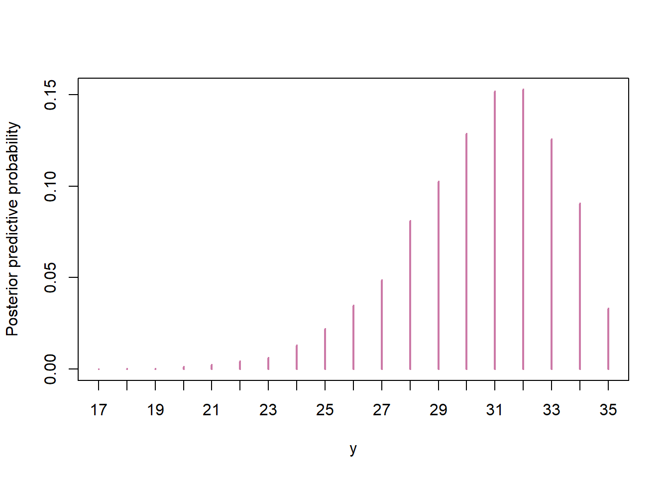
quantile(y_sim, c(0.025, 0.975))## 2.5% 97.5% ## 24 35The interval is similar to the one from the grid approximation, and the interpretation is the same. There is posterior predictive probability of 95% that between 24 and 35 students in a sample of 35 students will prefer data as singular.
You can tune the shape parameters — \(\alpha\) (like “prior successes”) and \(\beta\) (like “prior failures”) — of a Beta distribution to your prior beliefs in a few ways. Recall that \(\kappa = \alpha + \beta\) is the “concentration” or “equivalent prior sample size”.
- If prior mean \(\mu\) and prior concentration \(\kappa\) are specified then \[\begin{align*} \alpha &= \mu \kappa\\ \beta & =(1-\mu)\kappa \end{align*}\]
- If prior mode \(\omega\) and prior concentration \(\kappa\) (with \(\kappa>2\)) are specified then \[\begin{align*} \alpha &= \omega (\kappa-2) + 1\\ \beta & = (1-\omega) (\kappa-2) + 1 \end{align*}\]
- If prior mean \(\mu\) and prior sd \(\sigma\) are specified then \[\begin{align*} \alpha &= \mu\left(\frac{\mu(1-\mu)}{\sigma^2} -1\right)\\ \beta & = \left(1-\mu\right)\left(\frac{\mu(1-\mu)}{\sigma^2} -1\right) %\beta & = \alpha\left(\frac{1}{\mu} - 1\right)\\ \end{align*}\]
- You can also specify two percentiles and use software to find \(\alpha\) and \(\beta\). For example, you could specify the endpoints of a prior 98% credible interval.
- Sketch your Beta prior distribution for \(\theta\). Describe its main features and your reasoning. Then translate your prior into a Beta distribution by specifying the shape parameters \(\alpha\) and \(\beta\).
- Assume a prior Beta distribution for \(\theta\) with prior mean 0.15 and prior SD is 0.08. Find \(\alpha\) and \(\beta\), and a prior 98% credible interval for \(\theta\).
- Of course, choices will vary, based on what you know about left-handedness. But do think about what your prior might look like, and use one of the methods to translate it to a Beta distribution.
- Let’s say we’ve heard that about 15% of people in general are left-handed, but we’ve also heard 10% so we’re not super sure, and we also don’t know how Cal Poly students compare to the general population. So we’ll assume a prior Beta distribution for \(\theta\) with prior mean 0.15 (our “best guess”) and a prior SD of 0.08 to reflect our degree of uncertainty. This translates to a Beta(2.8, 16.1) prior, with a central 98% prior credible interval for \(\theta\) that between 2.2% and 38.1% of Cal Poly students are left-handed. We could probably go with more prior certainty than this, but it seems at least like a reasonable starting place before observing data. We can (and should) use prior predictive tuning to aid in choosing \(\alpha\) and \(\beta\) for our Beta distribution prior.
mu = 0.15
sigma = 0.08

alpha = mu ^ 2 * ((1 - mu) / sigma ^ 2 - 1 / mu); alpha
## [1] 2.838beta <- alpha * (1 / mu - 1); beta## [1] 16.08qbeta(c(0.01, 0.99), alpha, beta)## [1] 0.02222 0.38104