3.3 Working with probabilities
In the previous section we encountered two interpretations of probability: long run relative frequency and subjective. We will use these interpretations interchangeably. With subjective probabilities it is often helpful to consider what might happen in a simulation. It is also useful to consider long run relative frequencies in terms of relative degrees of likelihood. Fortunately, the mathematics of probability work the same way regardless of the interpretation.
3.3.1 Consistency requirements
With either the long run relative frequency or subjective probability interpretation there are some basic logical consistency requirements which probabilities need to satisfy. Roughly, probabilities cannot be negative and the sum of probabilities over all possible outcomes must be 100%.
Example 3.3 As of Dec 30, FiveThirtyEight listed the following probabilities for who will win the 2022 Superbowl.
| Team | Probability |
|---|---|
| Kansas City Chiefs | 26% |
| Green Bay Packers | 24% |
| Tampa Bay Buccaneers | 9% |
| Dallas Cowboys | 8% |
| Other |
According to FiveThirtyEight (as of Dec 30):
- What would you expect the results of 10000 repetitions of a simulation of the Superbowl champion to look like? Construct a table summarizing what you expect. Is this necessarily what would happen?
- What must be the probability that the Chiefs do not win the 2022 Superbowl?
- What must be the probability that one of the above four teams is the Superbowl champion?
- What must be the probability that a team other than the above four teams is the Superbowl champion? That is, what value goes in the “Other” row in the table?
\iffalse{} Solution. to Example 3.3
Show/hide solution
While these particular probabilities are subjective, imagining probabilities as relative frequencies often helps our intuition. If we think of this as a simulation, each repetition results in a World Series champion and in the long run we would expect the Dodgers would be the champion in 22%, or 2200, of the 10000 repetitions. We would expect the simulation results to look like
Team Repetitions as winner Kansas City Chiefs 2600 Green Bay Packers 2400 Tampa Bay Buccaneers 900 Dallas Cowboys 800 Other 3300 Of course, there would be some variability from simulation to simulation, just like in the sets of 1000 coin flips in Figure 3.4. But the above counts represent about what we would expect.
74%. Either the Chiefs win or they don’t; if there’s a 26% chance that the Chiefs win, there must be a 74% chance that they do not win. If we think of this as a simulation with 10000 repetitions, each repetition results in either the Chiefs winning or not, so if they win in 2600 of repetitions then they must not win in the other 7400.
67%. There is only one Superbowl champion, so if say the Chiefs win then no other team can win. Thinking again of the simulation, the repetitions in which the Chiefs win are distinct from those in which the Cowboys win. So if the Chiefs win in 2600 repetitions and the Cowboys win in 800 repetitions, then on a total of 3400 repetitions either the Chiefs or Cowboys win. Adding the four probabilities, we see that the probability that one of the four teams above wins must be 67%.
33%. Either one of the four teams above wins, or some other team wins. If one of the four teams above wins in 6700 repetitions, then in 3300 repetitions the winner is not one of these four teams.
Example 3.4 Suppose your subjective probabilities for the 2022 Superbowl champion satisfy the following conditions.
- The Cowboys and Buccaneers are equally likely to win
- The Packers are 1.5 times more likely than the Cowboys to win
- The Chiefs are 2 times more likely than the Packers to win
- The winner is as likely to be among these four teams — Chiefs, Packers, Buccaneers, Cowboys — as not
Construct a table of your subjective probabilities like the one in Example 3.3.
\iffalse{} Solution. to Example 3.4
Show/hide solution
Here, probabilities are specified indirectly via relative likelihoods. We need to find probabilities that are in the given ratios and add up to 100%. It helps to designate one outcome as the “baseline”. It doesn’t matter which one; we’ll choose the Cowboys.
- Suppose the Cowboys account for 1 “unit”. It doesn’t really matter what a unit is, but let’s say it corresponds to 1000 repetitions of the simulation. That is, the Cowboys win in 1000 repetitions. Careful: we haven’t yet specified how many total repetitions we have done, or how many units the entire simulation accounts for. We’re just starting with a baseline of what happens for the Cowboys.
- The Cowboys and Buccaneers are equally like to win, so the Buccaneers also account for 1 unit.
- The Packers are 1.5 times more likely than the Cowboys to win, so the Packers account for 1.5 units. If 1 unit is 1000 repetitions, then the Packers win in 1500 repetitions, 1.5 times more often than the Cowboys.
- The Chiefs are 2 times more likely than the Packers to win, so the Chiefs account for \(2\times 1.5=3\) units. If 1 unit is 1000 repetitions, then the Chiefs win in 3000 repetitions.
- The four teams account for a total of \(1+1+1.5+3 = 6.5\) units. Since the winner is as likely to among these four teams as not, then “Other” also accounts for 6.5 units.
- In total, there are 13 units which account for 100% of the probability. The Cowboys account for 1 unit, so their probability of winning is \(1/13\) or about 7.7%. Likewise, the probability that the Chiefs win is \(3/13\) or about 23.1%.
| Team | Units | Repetitions | Probability |
|---|---|---|---|
| Kansas City Chiefs | 3.0 | 3000 | 23.1% |
| Green Bay Packers | 1.5 | 1500 | 11.5% |
| Tampa Bay Buccaneers | 1.0 | 1000 | 7.7% |
| Dallas Cowboys | 1.0 | 1000 | 7.7% |
| Other | 6.5 | 6500 | 50.0% |
| Total | 13.0 | 13000 | 100.0% |
You should verify that all of the probabilities are in the specified ratios. For example, the Chiefs are 2 times more likely (\(2 = 23.1 / 11.5\)) than the Packers to win, and the Packers are 1.5 times more likely \((1.5 \approx 11.5 / 7.7)\) than the Cowboys to win.
We could have also solved this problem using algebra. Let \(x\) be the probability, as a decimal, that the Cowboys are the winner. (Again, it doesn’t matter which team is the baseline.) Then \(x\) is also the probability that the Buccaneers are the winner, \(1.5x\) for the Packers, and \(3x\) for the Chiefs. The probability that one of the four teams wins is \(x + x + 1.5x + 3x = 6.5x\), so the probability of Other is also \(6.5x\). The probabilities in decimal form must sum to 1 (that is, 100%), so \(1 = x + x + 1.5x + 3x + 6.5x = 13x\). Solve for \(x=1/13\) and then plug in \(x=1/13\) to find the other probabilities.
Example 3.4 illustrates one way of formulating probabilities. We start by specifying probabilities in relative terms, and then “normalize” these probabilities so that they add up to 100% while maintaining the ratios. As in the example, it helps to consider one outcome as a “baseline” and to specify all likelihoods relative to the baseline.
Figure 3.6 provides a visual representation of Example 3.4. The ratios provided in the problem setup are enough to draw the shape of the plot, represented by the plot on the left without a scale on the vertical axis. The heights are equal for the Cowboys and Buccaneers, the height for the Packers is 1.5 times higher, etc. The plot on the right simply adds a probability axis to ensure the values add to 1. The plot on the right represents the “normalization” step, but it does not affect the shape of the plot or the relative heights of the bars.
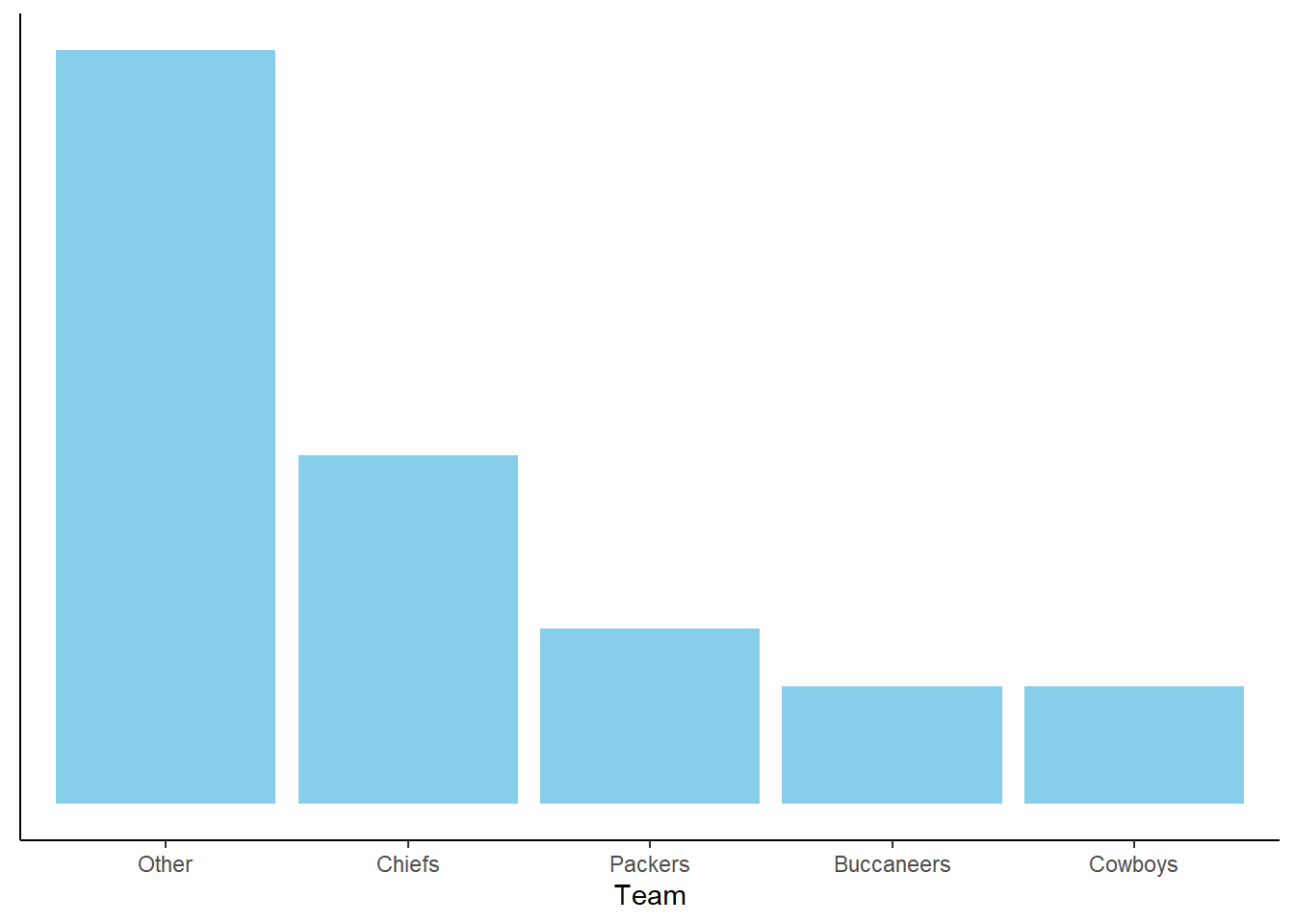
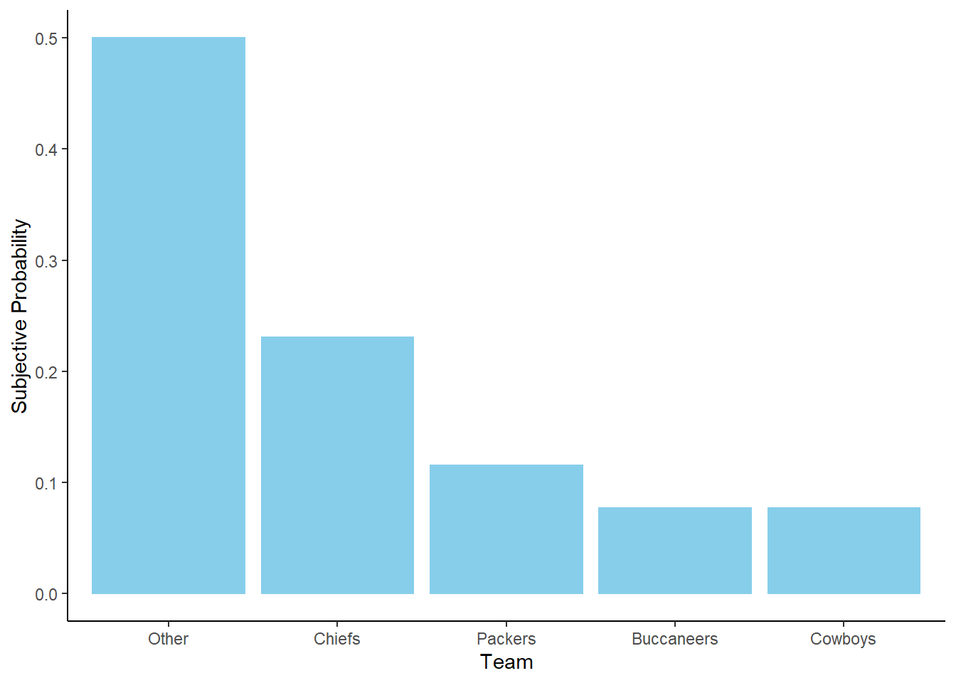
Figure 3.6: Bar chart representation of the subjective probabilities in Example 3.4. Left: Relative heights without absolute scale. Right: Heights scaled to sum to 1 to represent probabilities.