Chapter 12 Introduction to Bayesian Model Comparison
A Bayesian model is composed of both a model for the data (likelihood) and a prior distribution on model parameters. Model selection usually refers to choosing between different models for the data (likelihoods). But it can also concern choosing between models with the same likelihood but different priors.
In Bayesian model comparison, prior probabilities are assigned to each of the models, and these probabilities are updated given the data according to Bayes rule. Bayesian model comparison can be viewed as Bayesian estimation in a hierarchical model with an extra level for “model”. (We’ll cover hiearchical models in more detail later.)
Example 12.1 Suppose I have some trick coins, some of which are biased in favor of landing on heads, and some of which are biased in favor of landing on tails.20 I will select a trick coin at random; let \(\theta\) be the probability that the selected coin lands on heads in any single flip. I will flip the coin \(n\) times and use the data to decide about the direction of its bias. This can be viewed as a choice between two models
- Model 1: the coin is biased in favor of landing on heads
- Model 2: the coin is biased in favor of landing on tails
Assume that in model 1 the prior distribution for \(\theta\) is Beta(7.5, 2.5). Suppose in \(n=10\) flips there are 6 heads. Use simulation to approximate the probability of observing 6 heads in 10 flips given that model 1 is correct.
Assume that in model 2 the prior distribution for \(\theta\) is Beta(2.5, 7.5). Suppose in \(n=10\) flips there are 6 heads. Use simulation to approximate the probability of observing 6 heads in 10 flips given that model 2 is correct.
Use the simulation results to approximate and interpret the Bayes Factor in favor of model 1 given 6 heads in 10 flips.
Suppose our prior probability for each model was 0.5. Find the posterior probability of each model given 6 heads in 10 flips.
Suppose I know I have a lot more tail biased coins, so my prior probability for model 1 was 0.1. Find the posterior probability of each model given 6 heads in 10 flips.
Now suppose I want to predict the number of heads in the next 10 flips of the selected coin.
Use simulation to approximate the posterior predictive distribution of the number of heads in the next 10 flips given 6 heads in the first 10 flips given that model 1 is the correct model. In particular, approximate the posterior predictive probability that there are 7 heads in the next 10 flips given then model 1 is the correct model.
Repeat the previous part assuming model 2 is the correct model.
Suppose our prior probability for each model was 0.5. Use simulation to approximate the posterior predictive distribution of the number of heads in the next 10 flips given 6 heads in the first 10 flips. In particular, approximate the posterior predictive probability that there are 7 heads in the next 10 flips.
Given that model 1 is correct, simulate a value of \(\theta\) from a Beta(7.5, 2.5) prior, and then given \(\theta\) simulate a value of \(y\) from a Binomial(10, \(\theta\)) distribution. Repeat many times. The proportion of simulated repetitions that yield a \(y\) value of 6 approximates the probability of observing 6 heads in 10 flips given that model 1 is correct. The probability is 0.124.
Nrep = 1000000
theta = rbeta(Nrep, 7.5, 2.5)
y = rbinom(Nrep, 10, theta)
sum(y == 6) / Nrep
## [1] 0.1243Similar to he previous part, with the model 2 prior. The probability is 0.042.
Nrep = 1000000
theta = rbeta(Nrep, 2.5, 7.5)
y = rbinom(Nrep, 10, theta)
sum(y == 6) / Nrep
## [1] 0.04191The Bayes factor is the ratio of the likelihoods. The likelihood of 6 heads in 10 flips under model 1 is 0.124, and under model 2 is 0.042. The Bayes factor in favor of model 1 is 0.124/0.042 = 2.95. Observing 6 heads in 10 flips is 2.95 more likely under model 1 than under model 2. Also, the posterior odds in favor of model 1 given 6 heads in 10 flips are 2.95 times greater than the prior odds in favor of model 1.
In this case, the prior odds are 1, so the posterior odds in favor of model 1 are 2.95. The posterior probability of model 1 is 0.747, and the posterior probability of model 2 is 0.253.
Now the prior odds in favor of model 1 are 1/9. So the posterior odds in favor of model 1 given 6 heads in 10 flips are (1/9)(2.95)=0.328. The posterior probability of model 1 is 0.247, and the posterior probability of model 2 is 0.753.
Now suppose I want to predict the number of heads in the next 10 flips of the selected coin.
If model 1 is correct the prior is Beta(7.5, 2.5) so the posterior after observing 6 heads in 10 flips is Beta(13.5, 6.5). Simulate a value of \(\theta\) from a Beta(13.5, 6.5) distribution and given \(\theta\) simulate a value of \(y\) from a Binomial(10, \(\theta\)) distribution. Repeat many times. Approximate the posterior predictive probability of 7 heads in the 10 flips flips, given model 1 is correct and 6 heads in the first 10 flips, with the proportion of simulated repetitions that yield a \(y\) value of 7; the probability is 0.216.
Nrep = 1000000
theta = rbeta(Nrep, 7.5 + 6, 2.5 + 4)
y = rbinom(Nrep, 10, theta)
plot(table(y) / Nrep,
 ylab = "Posterior predictive probability",
 main = "Given Model 1")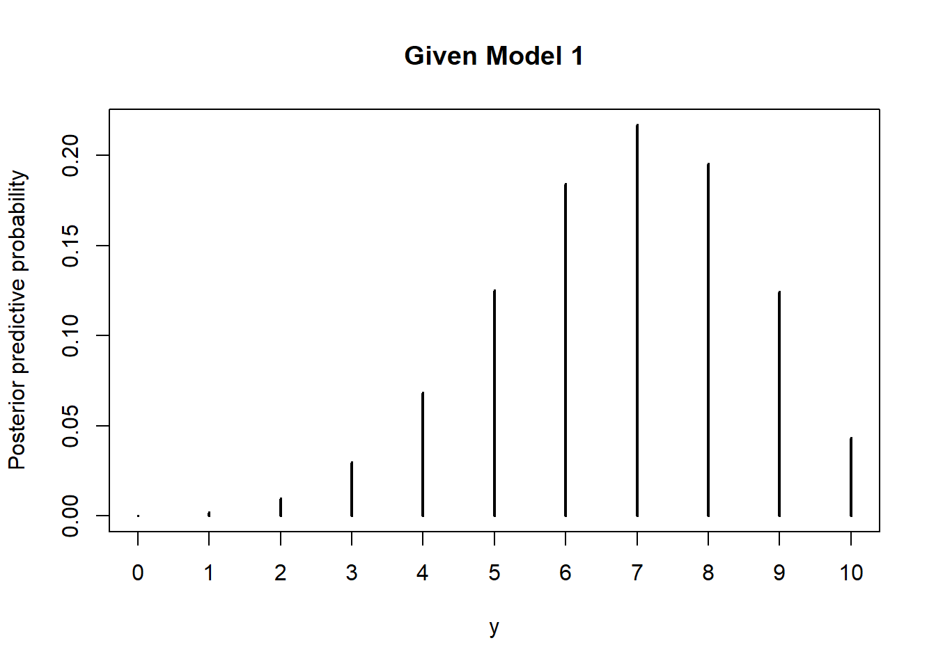
The simulation is similar, just use the prior in model 2. The posterior predictive probability of 7 heads in the 10 flips flips, given model 2 is correct and 6 heads in the first 10 flips, is 0.076.
Nrep = 1000000
theta = rbeta(Nrep, 2.5 + 6, 7.5 + 4)
y = rbinom(Nrep, 10, theta)
plot(table(y) / Nrep,
 ylab = "Posterior predictive probability",
 main = "Given model 2")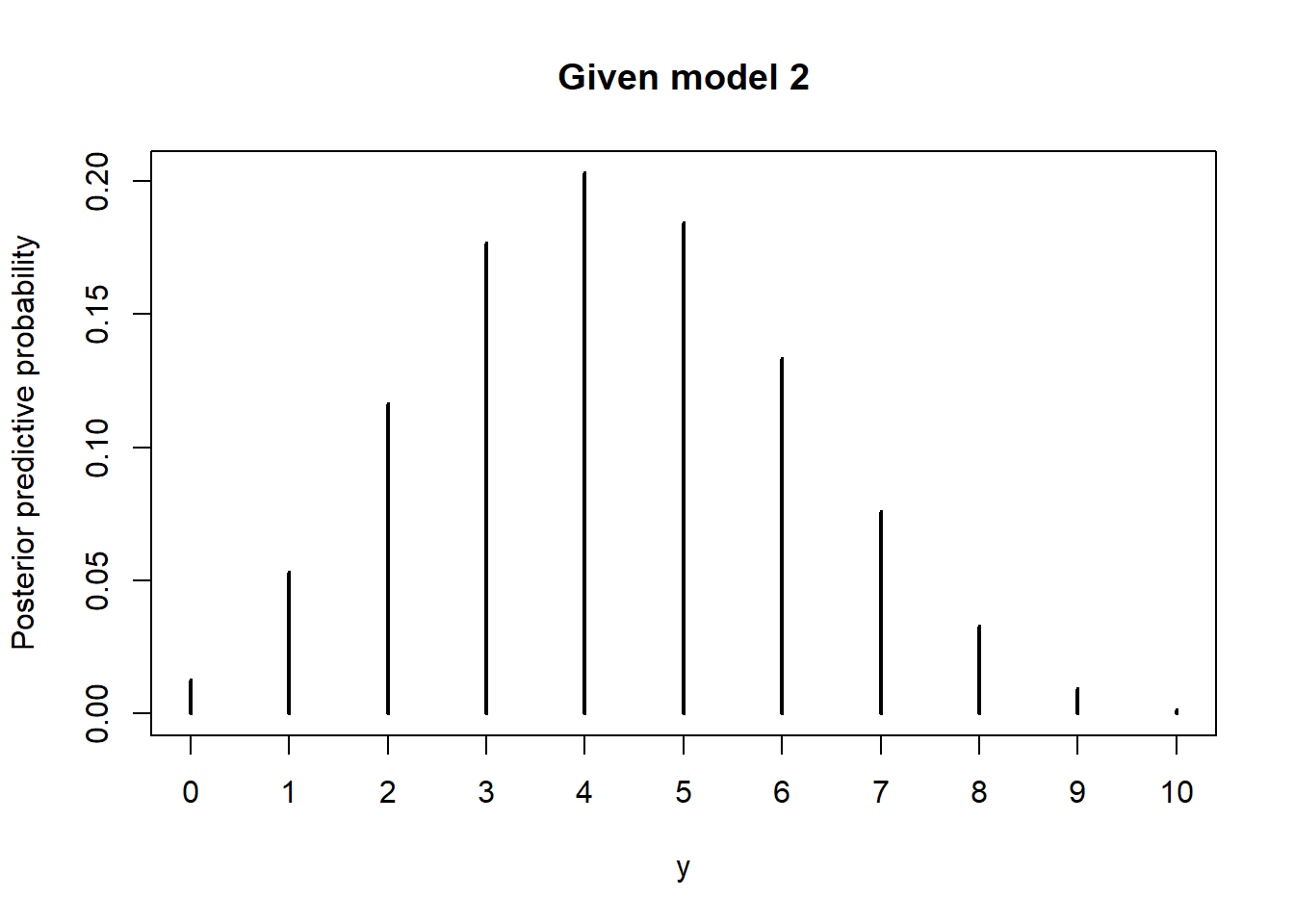
We saw in a previous part that with a 0.5/0.5 prior on model and 6 heads in 10 flips, the posterior probability of model 1 is 0.747 and of model 2 is 0.253. We now add another stage to our simulation
- Simulate a model: model 1 with probability 0.747 and model 2 with probability 0.253
- Given the model simulate a value of \(\theta\) from its posterior distribution: Beta(13.5, 6.5) if model 1, Beta(8.5, 11.5) if model 2.
- Given \(\theta\) simulate a value of \(y\) from a Binomial(10, \(\theta\)) distribtution
The simulation results are below. We can also find the posterior predictive probability of 7 heads in the next 10 flips using the law of total probability to combine the results from the two previous parts: \((0.747)(0.216)+(0.253)(0.076) = 0.18\)
Nrep = 1000000
alpha = c(7.5, 2.5) + 6
beta = c(2.5, 7.5) + 4

model = sample(1:2, size = Nrep, replace = TRUE, prob = c(0.747, 0.253))

theta = rbeta(Nrep, alpha[model], beta[model])

y = rbinom(Nrep, 10, theta)

plot(table(y) / Nrep,
 ylab = "Posterior predictive probability",
 main = "Model Average")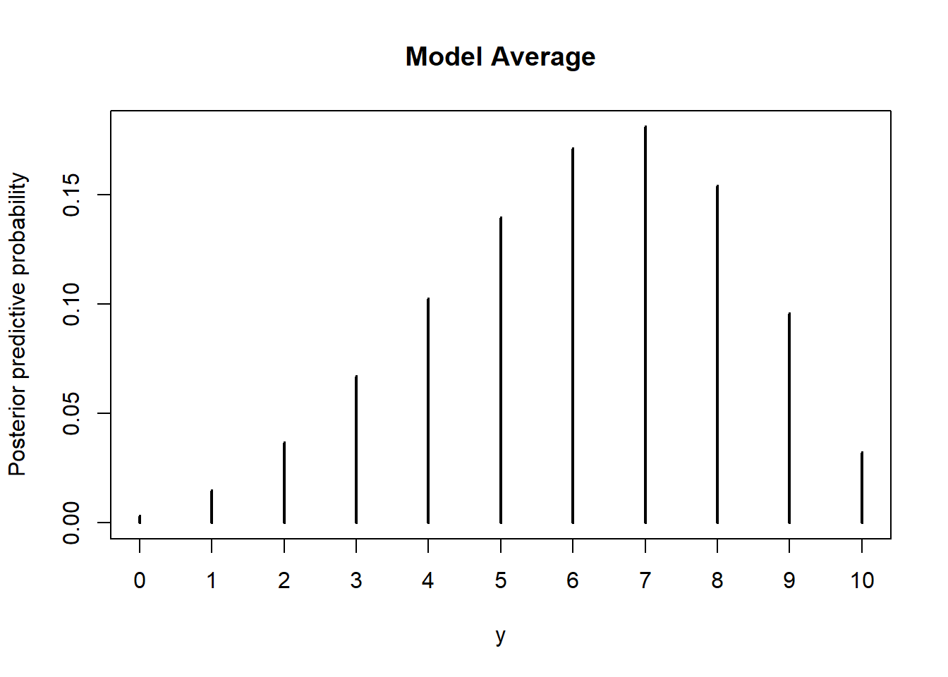
When several models are under consideration, the Bayesian model is the full hierarchical structure which spans all models being compared. Thus, the most complete posterior prediction takes into account all models, weighted by their posterior probabilities. That is, prediction is accomplished by taking a weighted average across the models, with weights equal to the posterior probabilities of the models. This is called model averaging.
Example 12.2 Suppose again I select a coin, but now the decision is whether the coin is fair. Suppose we consider the two models
- “Must be fair” model: prior distribution for \(\theta\) is Beta(500, 500)
- “Anything is possible” model: prior distribution for \(\theta\) is Beta(1, 1)
- Suppose we observe 15 heads in 20 flips. Use simulation to approximate the Bayes factor in favor of the “must be fair” model given 15 heads in 20 flips. Which model does the Bayes factor favor?
- Suppose we observe 11 heads in 20 flips. Use simulation to approximate the Bayes factor in favor of the “must be fair” model given 11 heads in 20 flips. Which model does the Bayes factor favor?
- The “anything is possible” model has any value available to it, including 0.5 and the sample proportion 0.55. Why then is the “must be fair” option favored in the previous part?
A sample proportion of 15/20 = 0.75 does not seem consistent with the “must be fair” model, so we expect the Bayes Factor to favor the “anything in possible” model.
The Bayes Factor is the ratio of the likelihoods (of 15/20). To approximate the likelihood of 15 heads in 20 flips for the “must be fair” model
- Simulate a value \(\theta\) from a Beta(500, 500) distribution
- Given \(\theta\), simulate a value \(y\) from a Binomial(20, \(\theta\)) distribution
- Repeat many times and the proportion of simulated repetitions that yield a \(y\) of 15.
Approximate the likelihood of 15 heads in 20 flips for the “anything is possible” model similarly. The Bayes factor is the ratio of the likelihoods, about 0.323 in favor of the “must be fair” model. That is, the Bayes factor favors the “anything is possible” model.
Nrep = 1000000

theta1 = rbeta(Nrep, 500, 500)
y1 = rbinom(Nrep, 20, theta1)

theta2 = rbeta(Nrep, 1, 1)
y2 = rbinom(Nrep, 20, theta2)

sum(y1 == 15) / sum(y2 == 15)
## [1] 0.3197Similar to the previous part but with different data; now we compute the likelihood of 11 heads in 20 flips. The Bayes factor is about 3.34. Thus, the Bayes factor favors the “must be fair” model.
sum(y1 == 11) / sum(y2 == 11)## [1] 3.328A central 99% prior credible interval for \(\theta\) based on the “must be fair” model is (0.459, 0.541), which does not include the sample proportion of 0.55. So you might think that the data would favor the “anything is possible” model. However, the numerator and denominator in the Bayes factor are average likelihoods: the likelihood of the data averaged over each possible value of \(\theta\). The “must be fair” model only gives initial plausibility to \(\theta\) values that are close to 0.5, and for such \(\theta\) values the likelihood of 11 heads in 20 flips is not so small. Values of \(\theta\) that are far from 0.5 are effectively not included in the average, due to their low prior probability, so the average likelihood is not so small.
In contrast, the “anything is possible” model stretches the prior probability over all values in (0, 1). For many \(\theta\) values in (0, 1) the likelihood of observing 11 heads in 20 flips is close to 0, and with the Uniform(0, 1) prior, each of these \(\theta\) values contributes equally to the average likelihood. Thus, the average likelihood is smaller for the “anything is possible” model than for the “must be fair” model.
Complex models generally have an inherent advantage over simpler models because complex models have many more options available, and one of those options is likely to fit the data better than any of the fewer options in the simpler model. However, we don’t always want to just choose the more complex model. Always choosing the more complex model overfits the data.
Bayesian model comparison naturally compensates for discrepancies in model complexity. In more complex models, prior probabilities are diluted over the many options available. Even if a complex model has some particular combination of parameters that fit the data well, the prior probability of that particular combination is likely to be small because the prior is spread more thinly than for a simpler model. Thus, in Bayesian model comparison, a simpler model can “win” if the data are consistent with it, even if the complex model fits well.
Example 12.3 Continuing Example 12.2 where we considered the two models
- “Must be fair” model: prior distribution for \(\theta\) is Beta(500, 500)
- “Anything is possible” model: prior distribution for \(\theta\) is Beta(1, 1)
Suppose we observe 65 heads in 100 flips.
Use simulation to approximate the Bayes factor in favor of the “must be fair” model given 65 heads in 100 flips. Which model does the Bayes factor favor?
We have discussed different notions of a “non-informative/vague” prior. We often think of Beta(1, 1) = Uniform(0, 1) as a non-informative prior, but there are other considerations. In particular, a Beta(0.01, 0.01) is often used a non-informative prior in this context. Think of a Beta(0.01, 0.01) prior like an approximation to the improper Beta(0, 0) prior based on “no prior successes or failures”.
Suppose now that the “anything is possible” model corresponds to a Beta(0.01, 0.01) prior distribution for \(\theta\). Use simulation to approximate the Bayes factor in favor of the “must be fair” model given 65 heads in 100 flips. Which model does the Bayes factor favor? Is the choice of model sensitive to the change of prior distribution within the “anything is possible” model?
For each of the two “anything is possible” priors, find the posterior distribution of \(\theta\) and a 98% posterior credible interval for \(\theta\) given 65 heads in 100 flips. Is estimation of \(\theta\) within the “anything is possible” model sensitive to the change in the prior distribution for \(\theta\)?
The simulation is similar to the ones in the previous example, just with different data. The Bayes Factor is about 0.126 in favor of the “must be fair” model. So the Bayes Factor favors the “anything is possible” model.
Nrep = 1000000

theta1 = rbeta(Nrep, 500, 500)
y1 = rbinom(Nrep, 100, theta1)

theta2 = rbeta(Nrep, 1, 1)
y2 = rbinom(Nrep, 100, theta2)

sum(y1 == 65) / sum(y2 == 65)
## [1] 0.1325The simulation is similar to the one in the previous part, just with a different prior. The Bayes Factor is about 5.73 in favor of the “must be fair” model. So the Bayes Factor favors the “must be fair” model. Even though there both non-informative priors, the Beta(1, 1) and Beta(0.01, 0.01) priors leads to very different Bayes factors and decisions. The choice of model does appear to be sensitive to the choice of prior distribution.
Nrep = 1000000

theta1 = rbeta(Nrep, 500, 500)
y1 = rbinom(Nrep, 100, theta1)

theta2 = rbeta(Nrep, 0.01, 0.01)
y2 = rbinom(Nrep, 100, theta2)

sum(y1 == 65) / sum(y2 == 65)
## [1] 5.272For a Beta(1, 1) prior, the posterior of \(\theta\) given 65 heads in 100 flips is the Beta(66, 36) distribution, and a central 98% posterior credible interval for \(\theta\) is (0.534, 0.752). For a Beta(0.01, 0.01) prior, the posterior of \(\theta\) given 65 heads in 100 flips is the Beta(65.01, 35.01) distribution, and a central 98% posterior credible interval for \(\theta\) is (0.536, 0.755). The Beta(66, 36) and Beta(65.01, 35.01) distributions are virtually identical, and the 98% credible intervals are practically the same. At least in this case, the estimation of \(\theta\) within the “anything is possible” model does not appear to be sensitive to the choice of prior.
qbeta(c(0.01, 0.99), 1 + 65, 1 + 35)## [1] 0.5340 0.7517qbeta(c(0.01, 0.99), 0.01 + 65, 0.01 + 35)## [1] 0.5359 0.7553
In Bayesian estimation of continuous parameters within a model, the posterior distribution is typically not too sensitive to changes in prior (provided that there is a reasonable amount of data and the prior is not too strict).
In contrast, in Bayesian model comparison, the posterior probabilities of the models and the Bayes factors can be extremely sensitive to the choice of prior distribution within each model.
When comparing different models, prior distributions on parameters within each model should be equally informed. One strategy is to use a small set of “training data” to inform the prior of each model before comparing.
Example 12.4 Continuing Example 12.3 where we considered two priors in the “anything is possible model”: Beta(1, 1) and Beta(0.1, 0.1). We will again compare the “anything is possible model” to the “must be fair” model which corresponds to a Beta(500, 500) prior.
Suppose we observe 65 heads in 100 flips.
- Assume the “anything is possible” model corresponds to the Beta(1, 1) prior. Suppose that in the first 10 flips there were 6 heads. Compute the posterior distribution of \(\theta\) in each of the models after the first 10 flips. Then use simulation to approximate the Bayes factor in favor of the “must be fair” model given 65 heads in 100 flips, using the posterior distribution of \(\theta\) after the first 10 flips as the prior distribution in the simulation. Which model does the Bayes factor favor?
- Repeat the previous part assuming the “anything is possible” model corresponds to the Beta(0.01, 0.01) prior. Compare with the previous part.
With the Beta(1, 1) prior in the “anything is possible” model, the posterior distribution of \(\theta\) after 6 heads in the first 10 flips is the Beta(7, 5) distribution. With the Beta(500, 500) prior in the “must be fair” model, the posterior distribution of \(\theta\) after 6 heads in the first 10 flips is the Beta(506, 504) distribution. The simulation to approximate the likelihood in each model is similar to before, but now we simulate \(\theta\) from its posterior distribution after the first 10 flips, and evaluate the likelihood of observing 59 heads in the remaining 90 flips. The Bayes factor is about 0.056 in favor of the “must be fair” model. So the Bayes Factor favors the “anything is possible” model.
Nrep = 1000000

theta1 = rbeta(Nrep, 500 + 6, 500 + 4)
y1 = rbinom(Nrep, 90, theta1)

theta2 = rbeta(Nrep, 1 + 6, 1 + 4)
y2 = rbinom(Nrep, 90, theta2)

sum(y1 == 59) / sum(y2 == 59)
## [1] 0.05509With the Beta(0.01, 0.01) prior in the “anything is possible” model, the posterior distribution of \(\theta\) after 6 heads in the first 10 flips is the Beta(6.01, 4.01) distribution. The simulation is similar to the previous part, just with the different distribution for \(\theta\) in the “anything is possible” model. The Bayes factor is about 0.057 in favor of the “must be fair” model, about the same as in the previous part. So the Bayes Factor favors the “anything is possible” model. Notice that after “training” the models on the first 10 observations, the model comparison is no longer so sensitive to the choice of prior within the “anything is possible” model.
Nrep = 1000000

theta1 = rbeta(Nrep, 500 + 6, 500 + 4)
y1 = rbinom(Nrep, 90, theta1)

theta2 = rbeta(Nrep, 0.01 + 6, 0.01 + 4)
y2 = rbinom(Nrep, 90, theta2)

sum(y1 == 59) / sum(y2 == 59)
## [1] 0.05941
Example 12.5 Consider a null hypothesis significance test of \(H_0:\theta=0.5\) versus \(H_1:\theta\neq 0.5\). How does this situation resemble the previous problem?
We could treat this as a problem of Bayesian model comparison. The null hypothesis corresponds to a prior distribution which places all prior probability on the null hypothesized value of 0.5. The alternative hypothesis corresponds to a prior distribution over the full range of possible values of \(\theta\). Given data, we could compute the posterior probability of each model and use that to make a decision regarding the hypotheses. However, there are infinitely many choices for the prior that corresponds to the alternative hypothesis, and we have already seen that Bayesian model comparison can be very sensitive to the choice of prior within in model.
A null hypothesis significance test can be viewed as a problem of Bayesian model selection in which one model has a prior distribution that places all its credibility on the null hypothesized value. However, is it really plausible that the parameter is exactly equal to the hypothesized value?
Unfortunately, this model-comparison (Bayes factor) approach to testing can be extremely sensitive to the choice of prior corresponding to the alternative hypothesis.
An alternative Bayesian approach to testing involves choosing a region of practical equivalence (ROPE). A ROPE indicates a small range of parameter values that are considered to be practically equivalent to the null hypothesized value.
- A hypothesized value is rejected — that is, declared to be not credible — if its ROPE lies outside a posterior credible interval (e.g., 99%) for the parameter.
- A hypothesized value is accepted for practical purposes if its ROPE contains the posterior credible interval (e.g., 99%) for the parameter.
How do you choose the ROPE? That determines on the practical application.
In general, traditional testing of point null hypotheses (that is, “no effect/difference”) is not a primary concern in Bayesian statistics. Rather, the posterior distribution provides all relevant information to make decisions about practically meaningful issues. Ask research questions that are important in the context of the problem and use the posterior distribution to answer them.