Chapter 15 Bayesian Analysis of a Numerical Variable

In this chapter we’ll continue our study of a single numerical variable. When the distribution of the measured variable is symmetric and unimodal, the population mean is often the main parameter of interest. However, the population SD also plays an important role.

In the previous section we assumed that the measured numerical variable followed a Normal distribution. That is, we assumed a Normal likelihood function. However, the assumption of Normality is not always justified, even when the distribution of the measured variable is symmetric and unimodal. In this chapter we’ll investigate an alternative to a Normal likelihood that is more flexible and robust to outliers and extreme values.

Example 15.1 In a previous assignment, we assumed that birthweights (grams) of human babies follow a Normal distribution with unknown mean $\mu$ and known SD $\sigma=600$. (1 pound ≈ 454 grams.) We assumed a Normal(3400, 100) (in grams, or Normal(7.5, 0.22) in pounds) prior distribution for $\mu$; this prior distribution places most of its probability on mean birthweight being between 7 and 8 pounds.

Now we’ll assume, more realistically, that $\sigma$ is unknown.

What does the parameter $\sigma$ represent? What is a reasonable prior mean for $\sigma$? What range of values of $\sigma$ will account for most of the prior probability?
Assume a Gamma prior distribution for $\sigma$ with mean 600 and SD 200; this is a Gamma distribution with shape parameter $\alpha = 600^2/200^2$ and rate parameter $600/200^2$. Also assume that $\mu$ and $\sigma$ are independent according to the prior distribution. Explain how you could use simulation to approximate the prior predictive distribution of birthweights. Run the simulation and summarize the results. Does the choice of prior seem reasonable?

The following summarizes data on a random sample²⁸ of 1000 live births in the U.S. in 2001.

data = read.csv("_data/birthweight.csv")
y = data$birthweight

hist(y, freq = FALSE, breaks = 50)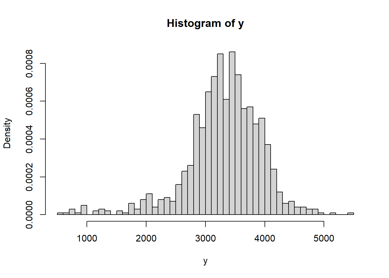

summary(y)

##    Min. 1st Qu.  Median    Mean 3rd Qu.    Max. 
##     595    3005    3350    3315    3714    5500

sd(y)

## [1] 631.3

n = length(y)
ybar = mean(y)

Does it seem reasonable to assume birthweights follow a Normal distribution?

Regardless of your answer to the previous question, continue to assume the model above. Use JAGS to find the posterior distribution.
How could you use simulation to approximate the posterior predictive distribution of birthweights? Run the simulation and find a 99% posterior prediction interval.
What percent of values in the observed sample fall outside the prediction interval? What does that tell you?

\iffalse{} Solution. to Example 15.1

The parameter $\sigma$ represents the population standard of individual birthweights: how much do birthweights vary from baby to baby? Our prior for $\mu$ says that a mean birthweight in the 7-8 or so pounds range seems reasonable. The parameter $\sigma$ represents how much individual birthweights vary about this mean. Let’s say that we think most babies weigh between 5 and 10 pounds; then we might want the interval [5, 10] to account for 95% of birthweights, or the values with 2 SDs of the mean, so we might want 5 pounds (the length of [5, 10]) to represent 4 SDs. So one reasonable prior mean of $\sigma$ might be around 1.25 pounds, or around 600 grams or so. Let’s choose a prior SD of 200 grams for $\sigma$ to cover a reasonably wide range of values of $\sigma$: values like 100 grams which represent little variability in birthweights, to values like 1000 grams which represent a great deal of variability in birthweights. That is, we’ll choose a Gamma prior distribution for $\sigma$ with mean 600 and SD 200; this is a Gamma distribution with shape parameter $\alpha = 600^2/200^2$ and rate parameter $600/200^2$. Remember, this is only one choice for prior. There are many other reasonable choices.
Simulate a value $\mu$ from a Normal(3400, 100) distribution, and independently simulate a value of $\sigma$ from a Gamma($600^2/200^2$, $600/200^2$) distribution. Given $\mu$ and $\sigma$, simulate a value $y$ from a Normal($\mu$, $\sigma$) distribution. Repeat many times and summarize the simulated $y$ values to approximate the prior predictive distribution. The results are below. According to this prior model, we predict that most babies weigh between about 4.5 and 10.5 pounds, which seems reasonable based on what we know about birthweights.
```
n_rep = 10000

mu_sim = rnorm(n_rep, 3400, sd = 100)

sigma_sim = rgamma(n_rep, 600 ^ 2 / 200 ^ 2, 600 / 200 ^2)

y_sim = rnorm(n_rep, mu_sim, sigma_sim)

hist(y_sim,
 breaks = 50,
 freq = FALSE,
 main = "Prior Predictive Distribution",
 xlab = "birthweight (grams)")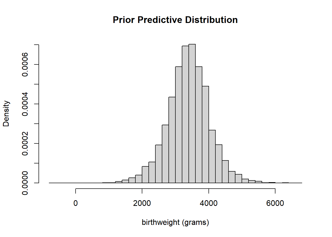
```
```
quantile(y_sim, c(0.025, 0.975))
```
```
##  2.5% 97.5% 
##  2086  4685
```
Assuming a Normal distribution doesn’t seem terrible, but it does appear that maybe the tails are a little heavier than we would expect for a Normal distribution, especially at the low birthweights. That is, there might be some evidence in the data that extremely low (and maybe high) birthweights don’t quite follow what would be expected if birthweights followed a Normal distribution.

See JAGS code below. A few notes:

The JAGS code takes the full sample of size 1000 as an input.
The data consists of 1000 values assumed to each be from a Normal($\mu$, $\sigma$) distribution.
Remember that in JAGS, it’s dnorm(mean, precision).
To find the likelihood of observing the entire sample, JAGS finds the likelihood of each of the individual values and then multiplies the values together for us to find the likelihood of the sample.
This is accomplished in JAGS by specifying the likelihood via a for loop which evaluates the likelihood y[i] ~ dnorm(mu, 1 / sigma ^ 2) for each y[i] in the sample.

Nrep = 10000
Nchains = 3

# data
# data has already been loaded in previous code
# y is the full sample
# n is the sample size

# model
model_string <- "model{

  # Likelihood
  for (i in 1:n){
y[i] ~ dnorm(mu, 1 / sigma ^ 2)
  }


  # Prior
  mu ~ dnorm(3400, 1 / 100 ^ 2)

  sigma ~ dgamma(600 ^ 2 / 200 ^ 2, 600 / 200 ^2)

}"

# Compile the model
dataList = list(y=y, n=n)

model <- jags.model(textConnection(model_string), 
                data=dataList,
                n.chains=Nchains)

## Compiling model graph
##    Resolving undeclared variables
##    Allocating nodes
## Graph information:
##    Observed stochastic nodes: 1000
##    Unobserved stochastic nodes: 2
##    Total graph size: 1017
## 
## Initializing model

update(model, 1000, progress.bar="none")

posterior_sample <- coda.samples(model, 
                             variable.names=c("mu", "sigma"),
                             n.iter=Nrep,
                             progress.bar="none")

# Summarize and check diagnostics
summary(posterior_sample)

## 
## Iterations = 2001:12000
## Thinning interval = 1 
## Number of chains = 3 
## Sample size per chain = 10000 
## 
## 1. Empirical mean and standard deviation for each variable,
##    plus standard error of the mean:
## 
##       Mean   SD Naive SE Time-series SE
## mu    3318 19.6   0.1130          0.113
## sigma  632 14.1   0.0813          0.102
## 
## 2. Quantiles for each variable:
## 
##       2.5%  25%  50%  75% 97.5%
## mu    3280 3305 3318 3331  3356
## sigma  605  622  631  641   660

plot(posterior_sample)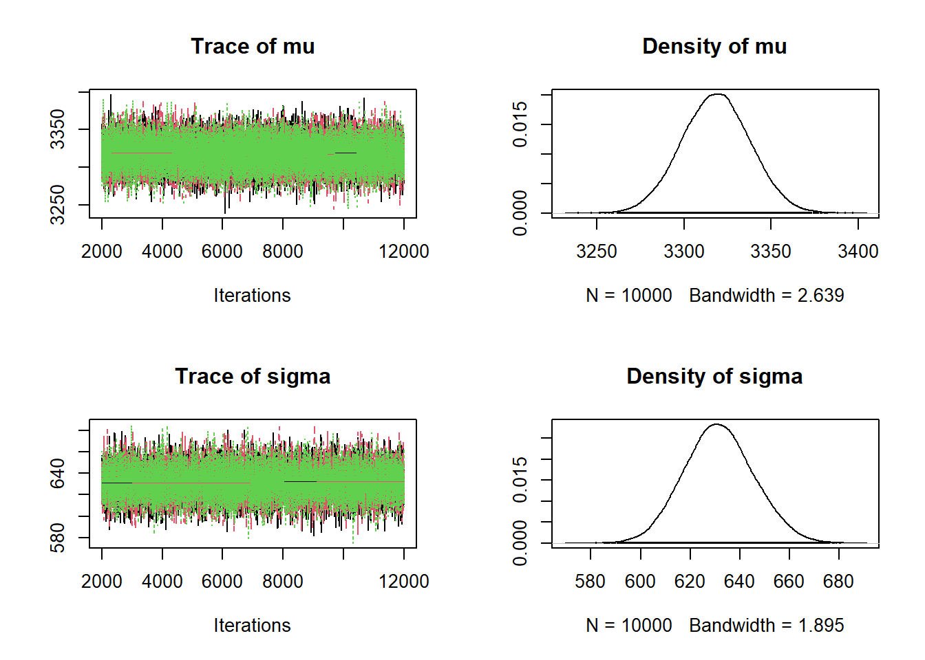

Simulate a $(\mu, \sigma)$ pair from the posterior distribution; JAGS has already done this for you. Then given $\mu$ and $\sigma$ simulate a value of $y$ from a Normal($\mu$, $\sigma$) distribution. Repeat many times and summarize the simulated values of $y$ to approximate the posterior predictive distribution of birthweights.
```
theta_sim = data.frame(as.matrix(posterior_sample))

y_sim = rnorm(Nrep, theta_sim$mu, theta_sim$sigma)

hist(y_sim, freq = FALSE, breaks = 50,
 xlab = "Birthweight (grams)",
 main = "Posterior predictive distribution")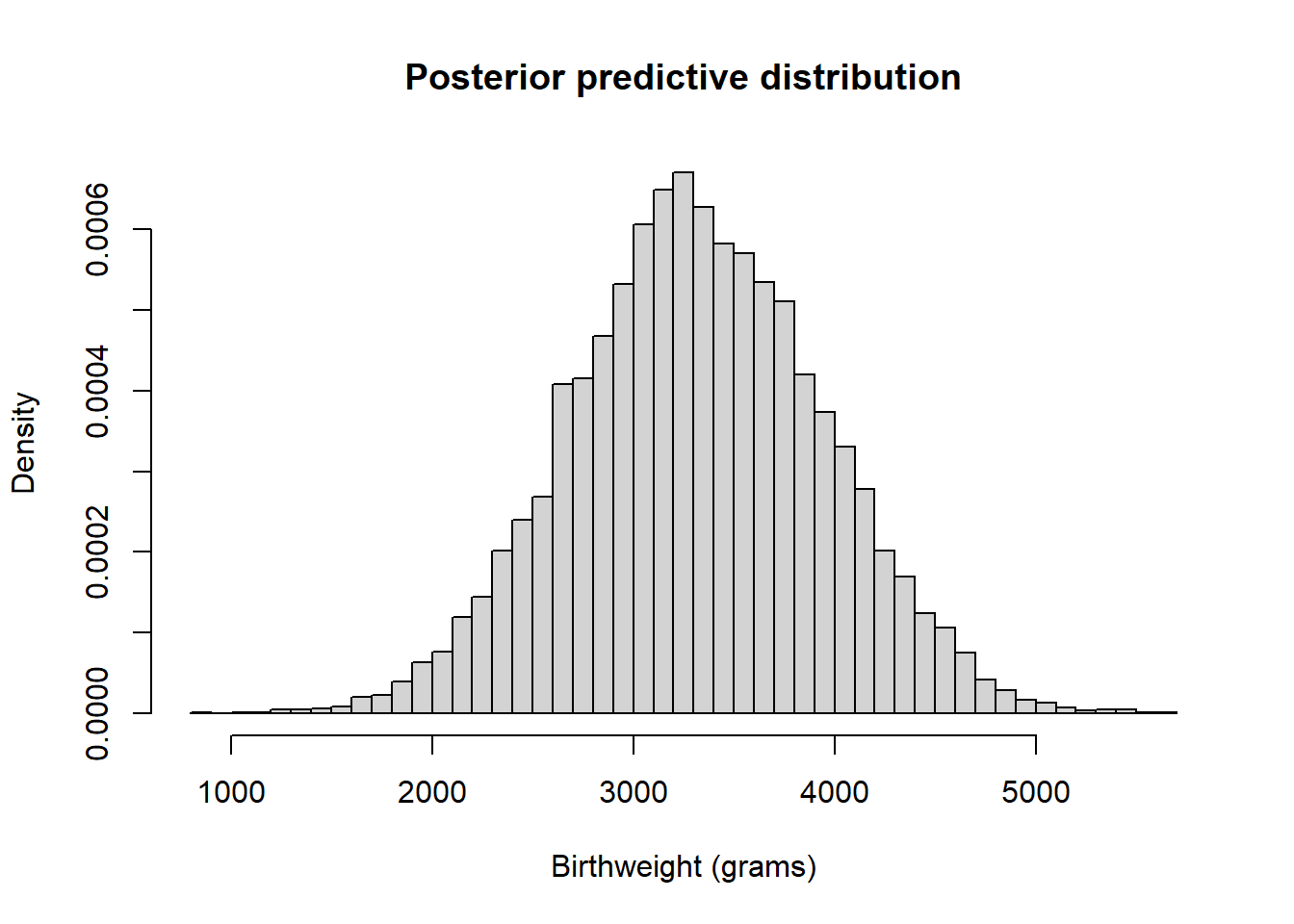
```
```
quantile(y_sim, c(0.005, 0.995))
```
```
##  0.5% 99.5% 
##  1703  4906
```
There is a posterior predictive probability of 99% that a randomly selected birthweight is between 1703 and 4906 grams. Roughly, this model and data say that 99% of birthweights are between 1703 and 4906 grams (3.8 and 10.8 pounds.).
Find the proportion of values in the observed sample that lie outside of the prediction interval
```
(sum(y < quantile(y_sim, 0.005)) + sum(y > quantile(y_sim, 0.995))) / n
```
```
## [1] 0.024
```
About 2.4 percent of birthweights in the sample fall outside of the 99% prediction interval, when we would only expect 1%. While not a large difference in magnitude, we are observing a higher percentage of birthweights in the tails than we would expect if birthweights followed a Normal distribution. So we have some evidence that a Normal model — that is, a Normal likelihood — might not be the best model for birthweights of all live births as it doesn’t properly account for extreme birthweights.

The code below performs a posterior predictive check by simulating hypothetical samples of size 1000 from the posterior model, and comparing with the observed sample of size 1000. The simulation is similar to the posterior predictive simulation in the previous example, but now every time we simulate a $(\mu, \sigma)$ pair, we simulate a random sample of 1000 $y$ values. Again, while not a terrible fit, there do seem to be more values in the tail — the lower tail especially — than would be expected under this model.

# plot the observed data
hist(y, freq = FALSE, breaks = 50) # observed data

# number of samples to simulate
n_samples = 100

# simulate (mu, sigma) pairs from the posterior
# we just randomly select rows from theta_sim 
index_sample = sample(Nrep, n_samples)

# simulate samples
for (r in 1:n_samples){
  
  i = index_sample[r]
  
  # simulate values from N(theta, sigma) distribution
  y_sim = rnorm(n, theta_sim[i, "mu"], theta_sim[i, "sigma"])
  
  # add plot of simulated sample to histogram
  lines(density(y_sim),
        col = rgb(135, 206, 235, max = 255, alpha = 25))
}

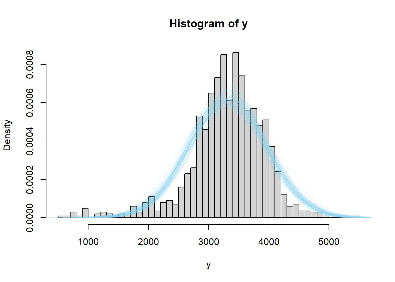
In the previous example we assumed a Normal likelihood. A Normal likelihood assumes that the population distribution of individual values of the measured numerical variable is Normal. Posterior predictive checking can be used to assess whether a Normal likelihood is appropriate for the observed data. If a Normal likelihood isn’t an appropriate model for the data then other likelihood functions can be used. In particular, if the observed data is relatively unimodal and symmetric²⁹ but has more extreme values than can be accommodated by a Normal likelihood, a $t$-distribution or other distribution with heavy tails can be used to model the likelihood.

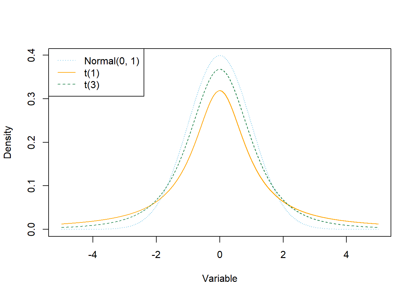
Normal distributions don’t allow much room for extreme values. An alternative is to assume a distribution with heavier tails. For example, t-distributions have heavier tails than Normal. For t-distributions, the degrees of freedom parameter $d \ge 1$ controls how heavy the tails are. When $d$ is small, the tails are much heavier than for a Normal distribution, leading to a higher frequency of extreme values. As $d$ increases, the tails get lighter and a $t$-distribution gets closer to a Normal distribution. For $d$ greater than 30 or so, there is very little different between a $t$-distribution and a Normal distribution except in the extreme tails. The degrees of freedom parameter $d$ is sometimes referred to as the “Normality parameter”, with larger values of $d$ indicating a population distribution that is closer to Normal.

Example 15.2 Continuing the birthweight example, we’ll now model the distribution of birthweights with a $t(\mu, \sigma, d)$ distribution.

How many parameters is the likelihood function based on? What are they?
What does assigning a prior distribution to the Normality parameter $d$ represent?
The Normality parameter must satisfy $d\ge 1$, so we want a distribution for which only values above 1 are possible. One way to accomplish this is to let $d_0 = d - 1$, assign a Gamma distribution prior to $d_0\ge 0$, and then let $d = 1 + d_0$. One common approach is to let the shape parameter of the Gamma distribution to be 1, and to let the scale parameter be 1/29, so that the prior mean of $d$ is 30. Assume the same priors for $\mu$ and $\sigma$ as in the previous example, and a Gamma(1, 1/29) prior for $(d-1)$. Use JAGS to fit the model to the birthweight data and approximate and summarize the posterior distribution.
Consider the posterior distribution for $d$. Based on this posterior distribution, is it plausible that birthweights follow a Normal distribution?
Consider the posterior distribution for $\sigma$. What seems strange about this distribution? (Hint: consider the sample SD.)
The standard deviation of a Normal($\mu$, $\sigma$) distribution is $\sigma$. However, the standard deviation of a $t(\mu, \sigma, d)$ distribution is not $\sigma$; rather it is $\sigma\sqrt{\frac{d}{d-2}}>\sigma$. When $d$ is large, $\sqrt{\frac{d}{d-2}}\approx 1$, and so the standard deviation is approximately $\sigma$. However, it can make a difference when $d$ is small.

Using the JAGS output, create a plot of the posterior distribution of $\sigma\sqrt{\frac{d}{d-2}}$. Does this posterior distribution of the population standard deviation seem more reasonable in light of the sample data?
How could you use simulation to approximate the posterior predictive distribution of birthweights? Run the simulation and find a 99% posterior prediction interval. How does it compare to the predictive interval from the model with the Normal likelihood?

\iffalse{} Solution. to Example 15.2

The $t(\mu, \sigma, d)$ is based on 3 parameters: the population mean $\mu$, the variability parameter $\sigma$ (which is NOT the population SD; see below), and the Normality parameter $d$.
Assigning a prior distribution to $d$ allows for a posterior distribution of $d$, which quantifies uncertainty about the degree of Normality versus “heavy-tailed-ness” of the distribution of birthweights. Assigning a prior distribution on $d$ allows the model to explore different values of $d$ to see what values seem most plausible given the observed data.

See the JAGS code below and output below. Note that the posterior distribution for $\mu$ is similar to the posterior distribution for $\mu$ from the model with the Normal likelihood.

Nrep = 10000
Nchains = 3

# data
# data has already been loaded in previous code
# y is the full sample
# n is the sample size

# model
model_string <- "model{

  # Likelihood
  for (i in 1:n){
y[i] ~ dt(mu, 1 / sigma ^ 2, tdf)
  }


  # Prior
  mu ~ dnorm(3400, 1 / 100 ^ 2)

  sigma ~ dgamma(600 ^ 2 / 200 ^ 2, 600 / 200 ^ 2)

  tdf <- 1 + tdf0

  tdf0 ~ dexp(1 / 29)

}"

# Compile the model
dataList = list(y=y, n=n)

model <- jags.model(textConnection(model_string), 
                data=dataList,
                n.chains=Nchains)

## Compiling model graph
##    Resolving undeclared variables
##    Allocating nodes
## Graph information:
##    Observed stochastic nodes: 1000
##    Unobserved stochastic nodes: 3
##    Total graph size: 1021
## 
## Initializing model

update(model, 1000, progress.bar="none")

posterior_sample <- coda.samples(model, 
                             variable.names=c("mu", "sigma", "tdf"),
                             n.iter=Nrep,
                             progress.bar="none")

# Summarize and check diagnostics
summary(posterior_sample)

## 
## Iterations = 2001:12000
## Thinning interval = 1 
## Number of chains = 3 
## Sample size per chain = 10000 
## 
## 1. Empirical mean and standard deviation for each variable,
##    plus standard error of the mean:
## 
##          Mean     SD Naive SE Time-series SE
## mu    3363.86 17.292  0.09983        0.12766
## sigma  467.18 17.753  0.10250        0.20309
## tdf      4.31  0.583  0.00336        0.00678
## 
## 2. Quantiles for each variable:
## 
##          2.5%    25%     50%     75%   97.5%
## mu    3329.69 3352.3 3363.82 3375.72 3397.52
## sigma  433.07  455.0  466.99  478.95  502.72
## tdf      3.34    3.9    4.25    4.65    5.61

plot(posterior_sample)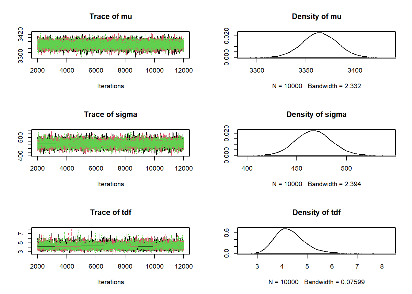

# Extract the JAGS output as a data frame
theta_sim = data.frame(as.matrix(posterior_sample))

The posterior distribution for $d$ places most of its probability on relatively small values of $d$. A 98% posterior credible interval for $d$ is 3.2 to 6. Values in this interval indicate relatively heavy tails in comparison to a Normal distribution. Therefore, the posterior distribution indicates that it is not plausible that birthweights follow a Normal disttribution.
The posterior distribution for $\sigma$ might seem initially strange. The sample standard is 631, but this value is not included the range of plausible values of $\sigma$ according to the posterior. This is an artifact of the interplay between $\sigma$ and $d$ in $t$-distributions, especially when $d$ is small. See the next part for more details.

See below. This posterior distribution seems more reasonable given the sample SD.

hist(theta_sim$sigma * sqrt(theta_sim$tdf / (theta_sim$tdf - 2)),
 freq = FALSE,
 breaks = 50,
 main = "Posterior distribution",
 xlab = expression(paste(sigma, " ", sqrt(frac(d, d-2)))))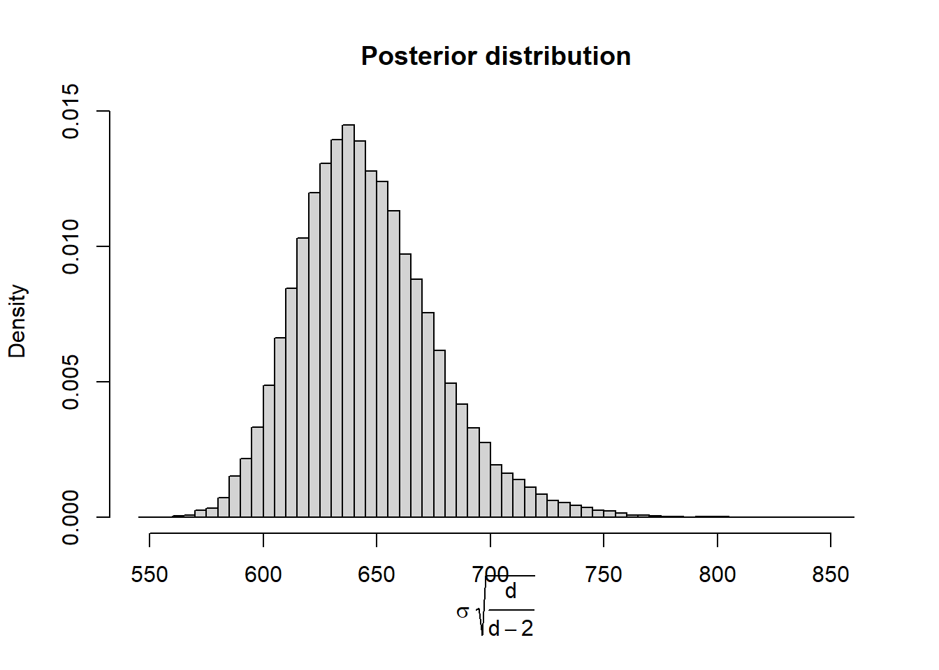

Simulate a triple $(\mu, \sigma, d)$ from the joint posterior distribution; JAGS has already done this for you. Given $(\mu, \sigma, d)$, simulate a value $y$ from a $t(\mu, \sigma, d)$ distribution. Repeat many times and summarize the simulated $y$ values to approximate the posterior distribution.

See the code and output below. The posterior predictive distribution now spans a more disperse range of birthweights that with the Normal model.
```
y_sim = theta_sim$mu + theta_sim$sigma * rt(Nrep, theta_sim$tdf)

hist(y_sim, freq = FALSE, breaks = 50,
 xlab = "Birthweight (grams)",
 main = "Posterior predictive distribution")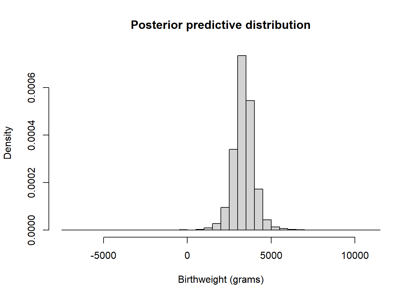
```
```
quantile(y_sim, c(0.005, 0.995))
```
```
##  0.5% 99.5% 
##  1236  5644
```

We’ll now try posterior predictive checks. We use the simulated values of $\theta$ from JAGS. For each value of $\theta$, we generate a sample of size 1000 from a t-distribution centered at $\theta$ and with a standard deviation of 600. (rt in R returns values on a standardized scale which we then rescale.)

# plot the observed data
hist(y, freq = FALSE, breaks = 50,
     ylim = c(0, 0.001)) # observed data

# number of samples to simulate
n_samples = 100

# simulate (mu, sigma, d) triples from the posterior
# we just randomly select rows from theta_sim 
index_sample = sample(Nrep, n_samples)

# simulate samples
for (r in 1:n_samples){
  
  # simulate values from a t-distribution
  y_sim = theta_sim[r, "mu"] + theta_sim[r, "sigma"] * rt(n, theta_sim[r, "tdf"])
  
  # add plot of simulated sample to histogram
  lines(density(y_sim),
        col = rgb(135, 206, 235, max = 255, alpha = 25))
}

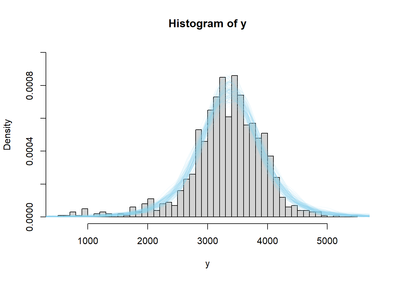
We see that the actual sample resembles simulated samples more closely for the model based on the t-distribution likelihood than for the one based on the Normal likelihood. While we do want a model that fits the data well, we also do not want to risk overfitting the data. In this case, we do not want a few extreme outliers to unduly influence the model. However, it does appear that a model that allows for heavier tails than a Normal distribution could be useful here. Moreover, accommodating the tails improves the fit in the center of the distribution too.

When the degrees of freedom are very small, $t$-distributions can give rise to super extreme values. We see this in the posterior predictive distribution for birthweights, where there are some negative birthweights and birthweights over 10000 grams. The model based on the the $t$-likelihood seems to fit well over the range of observed values of birthweight. As usual, we should refrain from making predictions outside the ranges of the observed data.

In models with multiple parameters, there can be dependencies between parameters, so interpreting the marginal posterior distribution of any single parameter can be difficult. It is often more helpful to consider predictive distributions, which accounts for the joint distribution of all parameters. Interpreting predictive distributions is often more intuitive since predictive distributions live on the scale of the measured variable.

The observational units in the examples in this section are live births. Many of the extremely low birthweights are attributed to babies who were born live but did not survive. Rather than model birthweights with one single likelihood, it might be more appropriate to first categorize the births and use the “group” variable in the model. For example, me might include a variable to indicate whether a baby is full term or not (or even just the length of the pregnancy). We will see how to compare a numerical variable across groups in upcoming sections.