Chapter 16 Comparing Two Samples

Most interesting statistical problems involve multiple unknown parameters. For example, many problems involve comparing two (or more) populations or groups based on two (or more) samples. In such situations, each population or group will have its own parameters, and there will often be dependence between parameters. We are usually interested in difference or ratios of parameters between groups.

The example below concerns the familiar context of comparing two means. However, the way independence is treated in the example is not the most common. Soon we will see hierarchical models for comparing groups.

Example 16.1 Do newborns born to mothers who smoke tend to weigh less at birth than newborns from mothers who don’t smoke? We’ll investigate this question using birthweight (pounds) data on a sample of births in North Carolina over a one year period.

Assume birthweights follow a Normal distribution with mean $\mu_1$ for nonsmokers and mean $\mu_2$ for smokers, and standard deviation $\sigma$.

Note: our primary goal will be to compare the means $\mu_1$ and $\mu_2$. We’re assuming a common standard deviation $\sigma$ to simplify a little, but we could (and probably should) also let standard deviation vary by smoking status.

The prior distribution will be a joint distribution on $(\mu_1, \mu_2, \sigma)$ triples. We could assume a prior under which $\mu_1$ and $\mu_2$ are independent. But why might we want to assume some prior dependence between $\mu_1$ and $\mu_2$? (For some motivation it might help to consider what the frequentist null hypothesis would be.)
One way to incorporate prior dependence is to assume a Multivariate Normal prior distribution. For the prior assume:
- $\sigma$ is independent of $(\mu_1, \mu_2)$
- $\sigma$ has a Gamma(1, 1) distribution
- $(\mu_1, \mu_2)$ follow a Bivariate Normal distribution with prior means (7.5, 7.5) pounds, prior standard deviations (0.5, 0.5) pounds, and prior correlation 0.9.
Simulate values of $(\mu_1, \mu_2)$ from the prior distribution³⁰ and plot them. Briefly³¹ describe the prior distribution.
How do you interpret the parameter $\mu_1 - \mu_2$? Plot the prior distribution of $\mu_1-\mu_2$, and find prior central 50%, 80%, and 98% credible interval. Also compute the prior probability that $\mu_1-\mu_2>0$.

The following code loads and summarizes the sample data. Briefly describe the data.

data = read.csv("_data/baby_smoke.csv")

ggplot(data, aes(weight, fill = habit)) + 
   geom_histogram(alpha = 0.3,
              aes(y = ..density..),
              position = 'identity')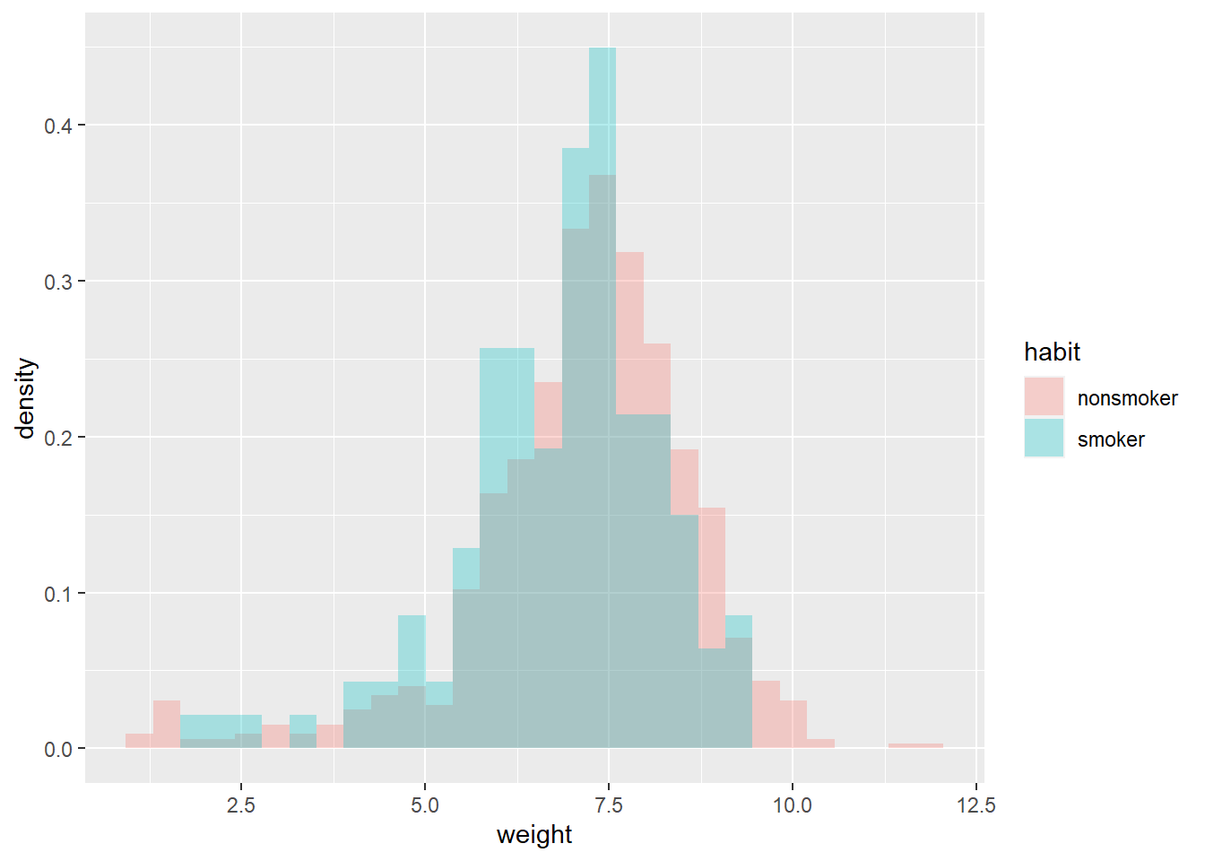

data %>%
  group_by(habit) %>%
  summarize(n(), mean(weight), sd(weight)) %>%
  kable(digits = 2)

habit	n()	mean(weight)	sd(weight)
nonsmoker	873	7.14	1.52
smoker	126	6.83	1.39

Is it reasonable to assume that the two samples are independent? (In this case the $y_1$ and $y_2$ samples would be conditionally independent given $(\mu_1, \mu_2, \sigma)$.)
Describe how you would compute the likelihood. For concreteness, how you would you compute the likelihood if there were only 4 babies in the sample: 2 non-smokers with birthweights of 8 pounds and 7 pounds, and 2 smokers with birthweights of 8.3 pounds and 7.1 pounds.
Use JAGS to approximate the posterior distribution. (The coding is a little tricky. See the code and some comments below.) Plot the posterior distribution. How strong is the dependence between $\mu_1$ and $\mu_2$ in the posterior? Why do you think that is?
Plot the posterior distribution of $\mu_1-\mu_2$ and describe it. Compute and interpret posterior central 50%, 80%, and 98% credible intervals. Also compute and interpret the posterior probability that $\mu_1-\mu_2>0$.
If we’re interested in $\mu_1-\mu_2$, why didn’t we put a prior directly on $\mu_1-\mu_2$ rather than on $(\mu_1,\mu_2)$?
Plot the posterior distribution of $\mu_1/\mu_2$, describe it, and find and interpret posterior central 50%, 80%, and 98% credible intervals.
Is there some evidence that babies whose mothers smoke tend to weigh less than those whose mothers don’t smoke?
Can we say that smoking is the cause of the difference in mean weights?
Is there some evidence that babies whose mothers smoke tend to weigh much less than those whose mothers don’t smoke? Explain.
One quantity of interest is the effect size, which is a way of measuring the magnitude of the difference between groups. When comparing two means, a simple measure of effect size (Cohen’s $d$) is \[ \frac{\mu_1 - \mu_2}{\sigma} \] Plot the posterior distribution of this effect size and describe it. Compute and interpret posterior central 50%, 80%, and 98% credible intervals.

\iffalse{} Solution. to Example 16.1

If our prior belief is that there is no difference in mean birthweights between babies of smokers and non-smokers, then our prior should place high probability on $\mu_1$ being close to $\mu_2$. Even if we want our prior to allow for different distributions for $\mu_1$ and $\mu_2$, there might still be some dependence. For example, we would assign a different prior conditional probability to the event that $\mu_1 > 8.5$ given $\mu_2 > 8.5$ than we would given $\mu_2<7.5$. Our prior uncertainty about mean birthweights of babies of nonsmokers informs our prior uncertainty about mean birthweights of babies in general, and hence also of babies of smokers.

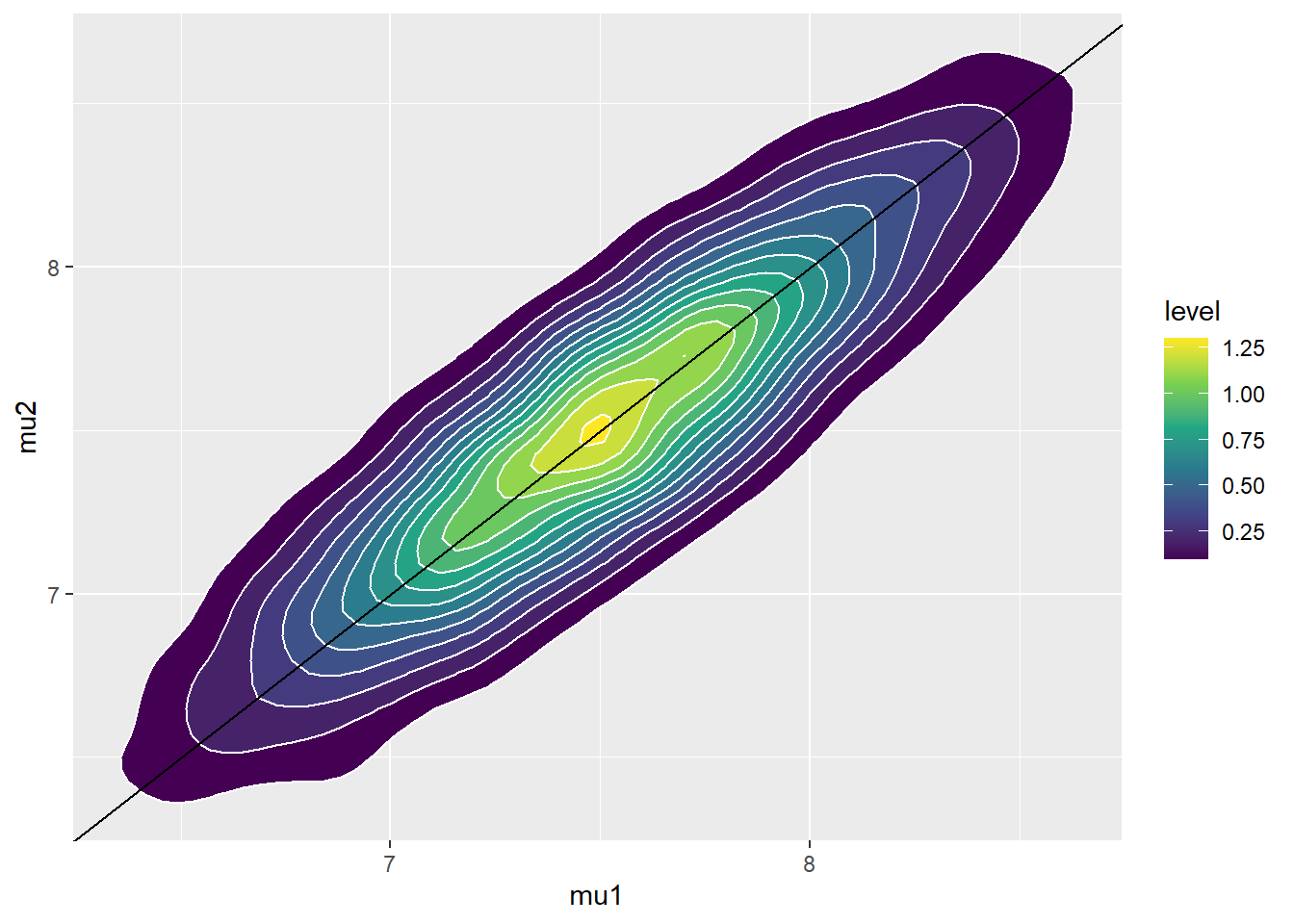
Our main focus is on $(\mu_1, \mu_2)$. We see that the prior places high density on $(\mu_1, \mu_2)$ pairs with $\mu_1$ close to $\mu_2$.

mu_prior_mean <- c(7.5, 7.5)
mu_prior_sd <- c(0.5, 0.5)
mu_prior_corr <- 0.9

mu_prior_cov <- matrix(c(mu_prior_sd[1] ^ 2,
              mu_prior_corr * mu_prior_sd[1] * mu_prior_sd[2],
              mu_prior_corr * mu_prior_sd[1] * mu_prior_sd[2],
              mu_prior_sd[2] ^ 2), nrow = 2)

library(MASS)

sim_prior = data.frame(mvrnorm(10000, mu_prior_mean, mu_prior_cov),
                           rgamma(10000, 1, 1))

names(sim_prior) = c("mu1", "mu2", "sigma")

ggplot(sim_prior, aes(mu1, mu2)) +
  geom_point(color = "skyblue", alpha = 0.4) +
  stat_ellipse(level = 0.98, color = "black", size = 2) +
  stat_density_2d(color = "grey", size = 1) +
  geom_abline(intercept = 0, slope = 1)

ggplot(sim_prior, aes(mu1, mu2)) +
  stat_density_2d(aes(fill = ..level..),
          geom = "polygon", color = "white") +
 scale_fill_viridis_c() +
  geom_abline(intercept = 0, slope = 1)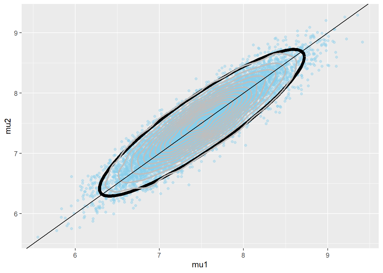

The parameter $\mu_1 - \mu_2$ is the difference in mean birthweights, smokers minus non-smokers. The prior mean of $\mu_1-\mu_2$ is 0, reflecting a prior belief towards no difference in mean birthweight between smokers and non-smokers. Furthermore, there is a fairly high prior probability that the mean birthweight for smokers is close to the mean birthweight for non-smokers, with a difference of at most about 0.5 pounds. Under this prior, nonsmokers and smokers are equally likely to have the higher mean birthweight.

sim_prior <- sim_prior %>%
  mutate(mu_diff = mu1 - mu2)

ggplot(sim_prior,
   aes(mu_diff)) +
  geom_histogram(aes(y=..density..), color = "black", fill = "white") +
  geom_density(size = 1, color = "skyblue") +
  labs(x = "Difference in population mean birthweight (pounds, non-smokers - smokers)",
   title = "Prior Distribution")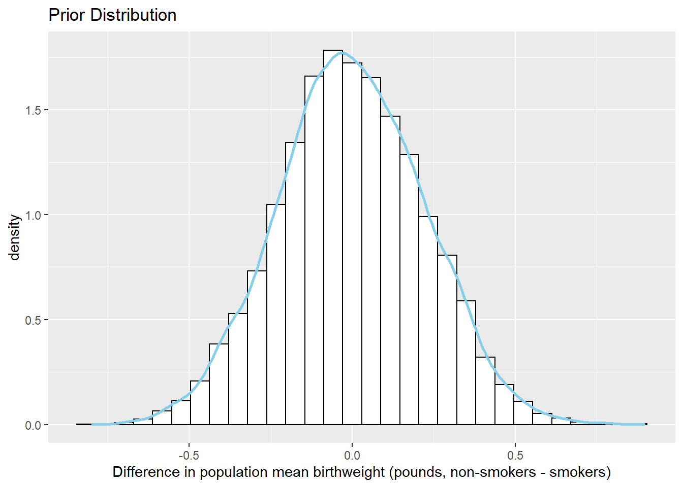

quantile(sim_prior$mu_diff, c(0.01, 0.10, 0.25, 0.75, 0.90, 0.99))

##      1%     10%     25%     75%     90%     99% 
## -0.5180 -0.2874 -0.1516  0.1503  0.2920  0.5161

sum(sim_prior$mu_diff > 0 ) / 10000

## [1] 0.4893

The distributions of birthweights are fairly similar for smokers and non-smokers. The sample mean birthweight for smokers is about 0.3 pounds less than the sample mean birthweight for smokers. The sample SDs of birthweights are similar for both groups, around 1.4-1.5 pounds.
Yes, it is reasonable to assume that the two samples are independent. The data for smokers was collected separately from the data for non-smokers. That is, it is reasonable to assume independence in the data.
For each observed value of birthweight for non-smokers, evaluate the likelihood based on a $N(\mu_1, \sigma)$ distribution. For example, if birthweight of a non-smoker is 8 pounds, the likelihood is dnorm(8, mu1, sigma); if birthweight of a non-smoker is 7 pounds, the likelihood is dnorm(7, mu1, sigma). The likelihood for the sample of non-smokers would be the products — assuming independence within sample — of the likelihoods of the individual values, as a function of $\mu_1$ and $\sigma$: dnorm(8, mu1, sigma) * dnorm(7, mu1, sigma) * ...

The likelihood for the sample of smokers would be the products of the likelihoods of the individual values, as a function of $\mu_2$ and $\sigma$: dnorm(8.3, mu2, sigma) * dnorm(7.1, mu2, sigma) * ...

The likelihood function for the full sample would be the product — assuming independence between samples — of the likelihoods for the two samples, a function of $\mu_1, \mu_2$ and $\sigma$.

Here is the code; there are some comments about syntax at the end of this chapter.

# data
y = data$weight

x = (data$habit == "smoker") + 1

n = length(y)

n_groups = 2

# Prior parameters
mu_prior_mean <- c(7.5, 7.5)
mu_prior_sd <- c(0.5, 0.5)
mu_prior_corr <- 0.9

mu_prior_cov <- matrix(c(mu_prior_sd[1] ^ 2,
              mu_prior_corr * mu_prior_sd[1] * mu_prior_sd[2],
              mu_prior_corr * mu_prior_sd[1] * mu_prior_sd[2],
              mu_prior_sd[2] ^ 2), nrow = 2)

# Model
model_string <- "model{

  # Likelihood
  for (i in 1:n){
  y[i] ~ dnorm(mu[x[i]], 1 / sigma ^ 2)
  }

  # Prior
  mu[1:n_groups] ~ dmnorm.vcov(mu_prior_mean[1:n_groups],
                           mu_prior_cov[1:n_groups, 1:n_groups])

  sigma ~ dgamma(1, 1)

}"

dataList = list(y = y, x = x, n = n, n_groups = n_groups,
            mu_prior_mean = mu_prior_mean, mu_prior_cov = mu_prior_cov)

# Compile
Nrep = 10000

n.chains = 5

model <- jags.model(textConnection(model_string),
                data = dataList,
                n.chains = n.chains)

## Compiling model graph
##    Resolving undeclared variables
##    Allocating nodes
## Graph information:
##    Observed stochastic nodes: 999
##    Unobserved stochastic nodes: 2
##    Total graph size: 2016
## 
## Initializing model

# Simulate
update(model, 1000, progress.bar = "none")

posterior_sample <- coda.samples(model,
                             variable.names = c("mu", "sigma"),
                             n.iter = Nrep,
                             progress.bar = "none")

sim_posterior = as.data.frame(as.matrix(posterior_sample))
names(sim_posterior) = c("mu1", "mu2", "sigma")
head(sim_posterior)

##     mu1   mu2 sigma
## 1 7.107 6.838 1.546
## 2 7.152 6.909 1.440
## 3 7.152 6.888 1.486
## 4 7.150 6.960 1.558
## 5 7.170 6.985 1.560
## 6 7.102 6.934 1.543

ggplot(sim_posterior, aes(mu1, mu2)) +
  geom_point(color = "seagreen", alpha = 0.4) +
  stat_ellipse(level = 0.98, color = "black", size = 2) +
  stat_density_2d(color = "grey", size = 1) +
  geom_abline(intercept = 0, slope = 1)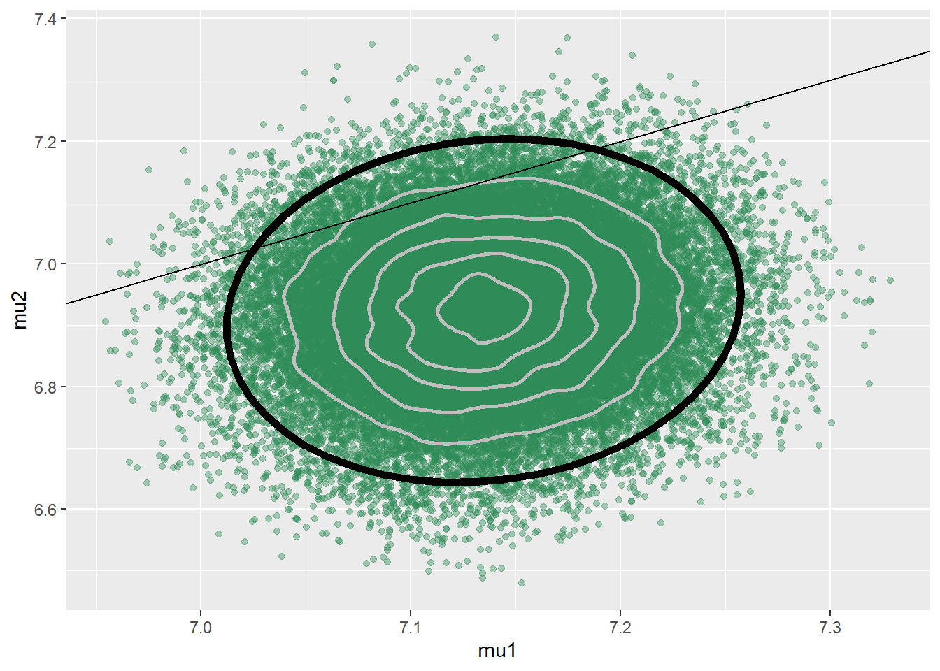

ggplot(sim_posterior, aes(mu1, mu2)) +
  stat_density_2d(aes(fill = ..level..),
          geom = "polygon", color = "white") +
 scale_fill_viridis_c() +
  geom_abline(intercept = 0, slope = 1)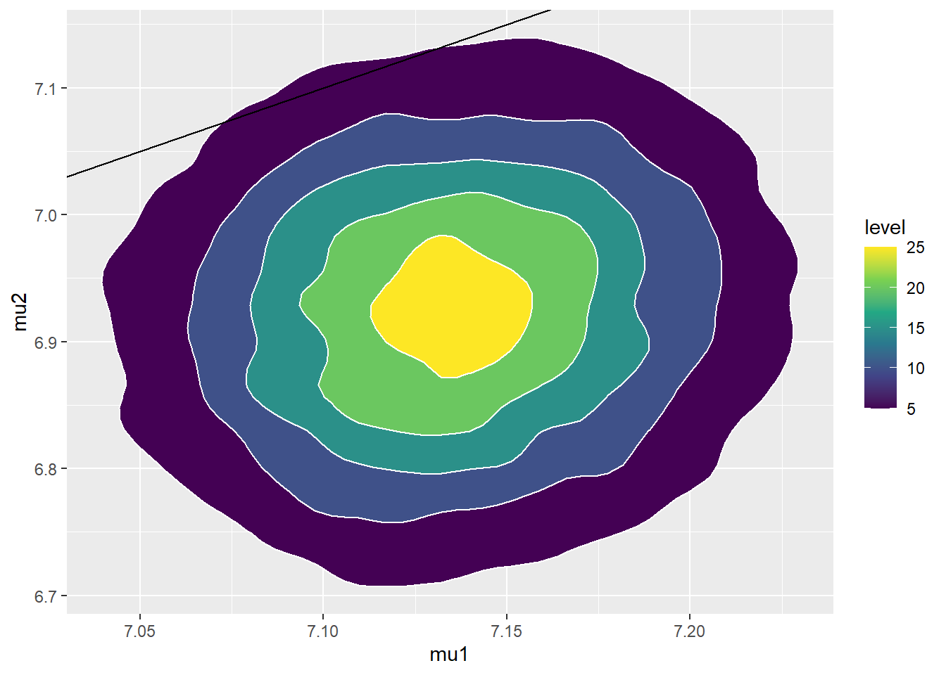

cor(sim_posterior$mu1, sim_posterior$mu2)

## [1] 0.09881

The posterior mean of $\mu_1$ is close to the sample mean birthweight for non-smokers, and the posterior mean of $\mu_2$ is close to the sample mean birthweight for smokers. The posterior SD of $\mu_1$ is smaller than that of $\mu_2$, reflecting the larger sample size for non-smokers than smokers. The posterior distribution places most of its probability on $(\mu_1, \mu_2)$ pairs with $\mu_1>\mu_2$, representing a much stronger belief (than prior) that mean birthweight for smokers is less than for non-smokers. The posterior correlation between $\mu_1$ and $\mu_2$ is about 0.1, which is much smaller than the prior correlation. Even though there was fairly strong dependence between $\mu_1$ and $\mu_2$ in the prior, there was independence between the samples in the data, represented in the likelihood. With the large sample sizes (especially for non-smokers) the data has more influence on the posterior than the prior does.

The code below summarizes the posterior distribution of the difference in means $\mu_1-\mu_2$. JAGS has already simulated $(\mu_1, \mu_2)$ pairs from the posterior distribution, so we just need to compute $\mu_1-\mu_2$ for each pair.
```
sim_posterior = sim_posterior %>%
  mutate(mu_diff = mu1 - mu2)

ggplot(sim_posterior,
   aes(mu_diff)) +
  geom_histogram(aes(y=..density..), color = "black", fill = "white") +
  geom_density(size = 1, color = "seagreen") +
  labs(x = "Difference in population mean birthweight (pounds, non-smokers - smokers)",
   title = "Posterior Distribution")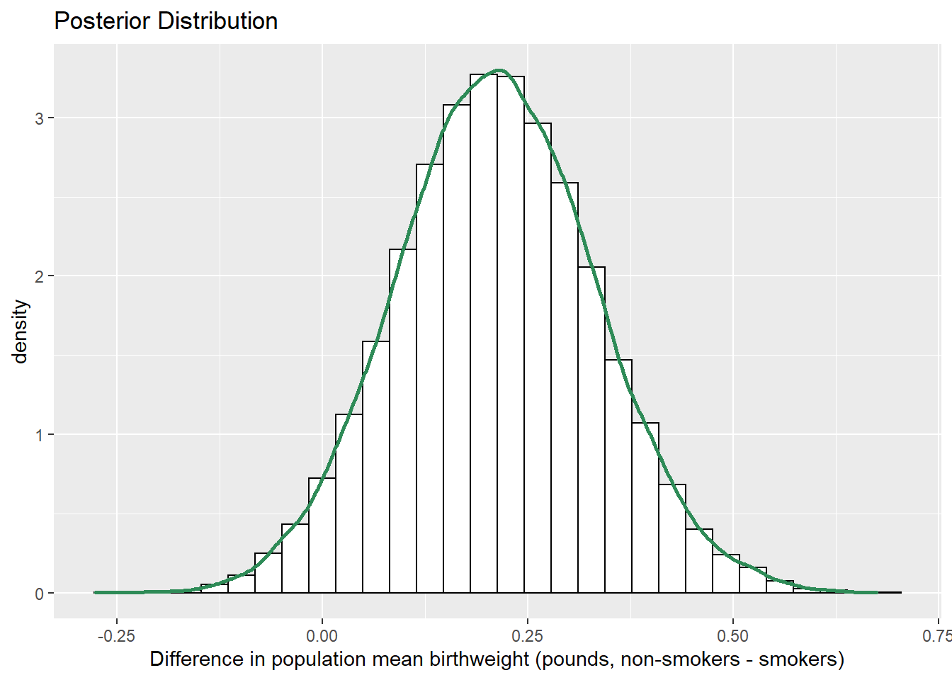
```
```
quantile(sim_posterior$mu_diff, c(0.01, 0.10, 0.25, 0.75, 0.90, 0.99))
```
```
##       1%      10%      25%      75%      90%      99% 
## -0.06321  0.05674  0.12952  0.29253  0.36675  0.50237
```
```
sum(sim_posterior$mu_diff > 0 ) / length(sim_posterior$mu_diff)
```
```
## [1] 0.961
```
The posterior distribution of $\mu_1-\mu_2$ is approximately Normal. The posterior mean of $\mu_1-\mu_2$ is about 0.21 pounds, which is a compromise between the prior mean of $\mu_1-\mu_2$ of 0 (no difference) and the difference in sample means of about 0.31 pounds.

There is a posterior probability of 50% that mean birthweight for non-smokers is between 0.13 and 0.29 pounds greater than mean birthweight for non-smokers.

There is a posterior probability of 80% that mean birthweight for non-smokers is between 0.06 and 0.37 pounds greater than mean birthweight for non-smokers.

There is a posterior probability of 98% that mean birthweight for non-smokers is between 0.06 pounds less and 0.5 pounds greater than mean birthweight for non-smokers.

There is a posterior probability of about 96 percent that the mean birthweight for non-smokers is greater than the mean birthweight for smokers.
Putting a prior directly on $\mu_1-\mu_2$ does allow us to make inference about the difference in mean birthweights. But what if we also want to estimate the mean birthweight for each group? Having a posterior distribution just on the difference between the two groups does not allow us to estimate the mean for either group. Also, $\mu_1-\mu_2$ is the absolute difference in means, but what if we want to measure the difference in relative terms? Putting a prior distribution on $(\mu_1, \mu_2)$ enables us to make posterior inference about mean birthweight for both non-smokers and smokers and any parameter (difference, ratio) that depends on the means.
See code and output below. JAGS has already simulated $(\mu_1, \mu_2)$ pairs from the posterior distribution, so we just need to compute $\mu_1/ \mu_2$ for each pair.
```
sim_posterior = sim_posterior %>%
  mutate(mu_ratio = mu1 / mu2)

ggplot(sim_posterior,
   aes(mu_ratio)) +
  geom_histogram(aes(y=..density..), color = "black", fill = "white") +
  geom_density(size = 1, color = "seagreen") +
  labs(x = "Ratio of population mean birthweight (non-smokers / smokers)",
   title = "Posterior Distribution")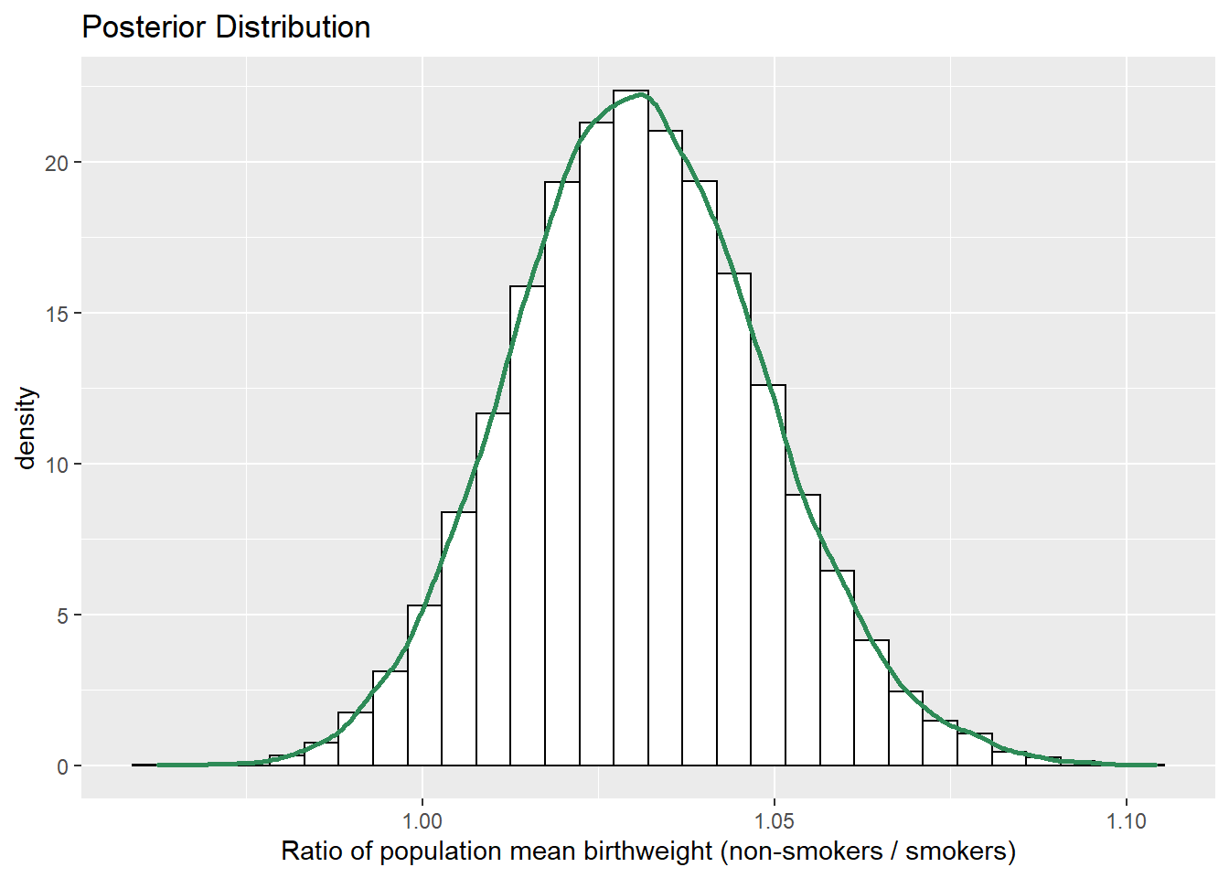
```
```
quantile(sim_posterior$mu_ratio, c(0.01, 0.10, 0.25, 0.75, 0.90, 0.99))
```
```
##     1%    10%    25%    75%    90%    99% 
## 0.9911 1.0080 1.0185 1.0427 1.0541 1.0754
```
The posterior distribution of $\mu_1/\mu_2$ is approximately Normal. The posterior mean of $\mu_1/\mu_2$ is about 1.03, which is a compromise between the prior mean of $\mu_1/\mu_2 = 1$ (no difference) and the ratio of sample means of 1.046.

There is a posterior probability of 50% that the mean birthweight of non-smokers is between 1.02 and 1.04 times greater than the mean birthweight of smokers.

There is a posterior probability of 80% that the mean birthweight of non-smokers is between 1.01 and 1.05 times greater than the mean birthweight of smokers.

There is a posterior probability of 98% that the mean birthweight of non-smokers is between 0.99 and 1.08 times greater than the mean birthweight of smokers.
Yes, there is some evidence. Even though we started with fairly strong prior credibility of no difference, with the relatively large sample sizes, the difference in sample means observed in the data was enough to overturn the prior beliefs. Now, the 98% credible interval for $\mu_1-\mu_2$ does contain 0, indicating some plausibility of no difference. But there’s nothing special about 98% credibility, and we should look at the whole posterior distribution. According to our posterior distribution, we place a high degree of plausibility on the mean birthweight for smokers being less than the mean birthweight of non-smokers.
The question of causation has nothing to do with whether we are doing a Bayesian or frequentist analysis. Rather, the question of causation concerns: how were the data collected? In particular, was this an experiment with random assignment of the explanatory variable? It wasn’t; it was an observational study (you can’t randomly assign some mothers to smoke). Therefore, there is potential for confounding variables. Maybe mothers who smoke tend to be less healthy in general than mothers who don’t smoke, and maybe some other aspect of health is more closely associated with lower birthweight than smoking is.
The posterior distribution of $\mu_1-\mu_2$ does not give much plausibility to large differences in mean birthweight. Almost all of the posterior probability is placed on the absolute difference being less than 0.5 pounds, and the relative difference being no more than 1.07 times. Just because we have evidence that there is a difference, doesn’t necessarily mean that the difference is large in practical terms.
The observed effect size is about 0.3/1.5 = 0.2. Birthweights vary naturally from baby to baby by about 1.5 pounds, so a difference of 0.3 pounds seems relatively small. The sample mean birthweight for non-smokers is 0.2 standard deviations greater than the sample mean birthweight for smokers.

The following simulates and summarizes the posterior distribution of the population effect size. JAGS has already simulated $(\mu_1, \mu_2, \sigma)$ triples for us; we just need to compute $(\mu_1 - \mu_2)/\sigma$ for each triple.
```
sim_posterior = sim_posterior %>%
  mutate(effect_size = (mu1 - mu2) / sigma)

ggplot(sim_posterior,
   aes(effect_size)) +
  geom_histogram(aes(y=..density..), color = "black", fill = "white") +
  geom_density(size = 1, color = "seagreen") +
  labs(x = "Effect size (non-smokers - smokers)",
   title = "Posterior Distribution")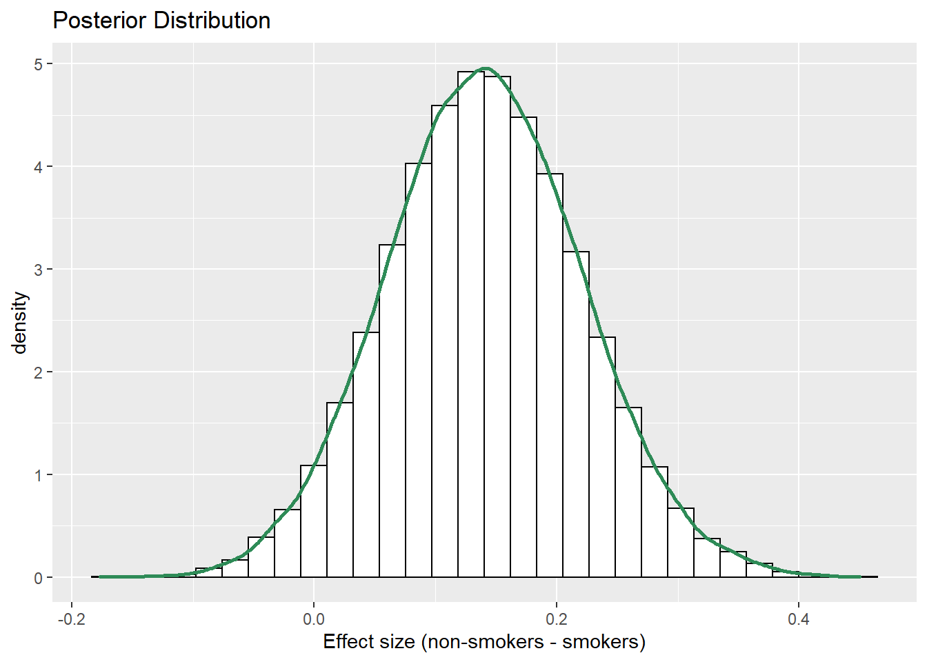
```
```
quantile(sim_posterior$effect_size, c(0.01, 0.10, 0.25, 0.75, 0.90, 0.99))
```
```
##       1%      10%      25%      75%      90%      99% 
## -0.04243  0.03773  0.08618  0.19465  0.24409  0.33520
```
The posterior mean of $(\mu_1-\mu_2)/\sigma$ is about 0.14, which is a compromise between the prior mean of $(\mu_1-\mu_2)/\sigma$ of 0 (no difference) and the sample effect size of 0.2.

There is a posterior probability of 50% that the mean birthweight of non-smokers is between 0.09 and 0.19 standard deviations greater than the mean birthweight of smokers.

There is a posterior probability of 80% that the mean birthweight of non-smokers is between 0.04 and 0.24 standard deviations greater than the mean birthweight of smokers.

There is a posterior probability of 98% that the mean birthweight of non-smokers is between 0.04 standard deviations less than and 0.34 standard deviations greater than the mean birthweight of smokers.

The posterior distribution indicates that the effect size is pretty small. The difference between mean birthweight of smokers and non-smokers is small relative to the variability in birthweights.

(Of course, smoking has many other adverse health effects. But looking at birthweight alone, based on this data set we cannot conclude that there is a large difference in mean birthweight between smokers and non-smokers.)

The previous example introduced many important ideas.

Independence in the data versus in the prior/posterior

It is typical to assume independence in the data, e.g., independence of values of the measured variables within and between samples (conditional on the parameters). Whether independence in the data is a reasonable assumption depends on how the data is collected.

But whether it is reasonable to assume prior independence of parameters is a completely separate question and is dependent upon our subjective beliefs about any relationships between parameters.

Transformations of parameters

The primary output of a Bayesian data analysis is the full joint posterior distribution on all parameters. Given the joint distribution, the distribution of transformations of the primary parameters is readily obtained.

Effect size for comparing means

When comparing groups, a more important question than “is there a difference?” is “how large is the difference?” An effect size is a measure of the magnitude of a difference between groups. A difference in parameters can be used to measure the absolute size of the difference in the measurement units of the variable, but effect size can also be measured as a relative difference.

When comparing a numerical variable between two groups, one measure of the population effect size is Cohens’s $d$ \[ \frac{\mu_1 - \mu_2}{\sigma} \]

The values of any numerical variable vary naturally from unit to unit. The SD of the numerical variable measures the degree to which individual values of the variable vary naturally, so the SD provides a natural “scale” for the variable. Cohen’s $d$ compares the magnitude of the difference in means relative to the natural scale (SD) for the variable

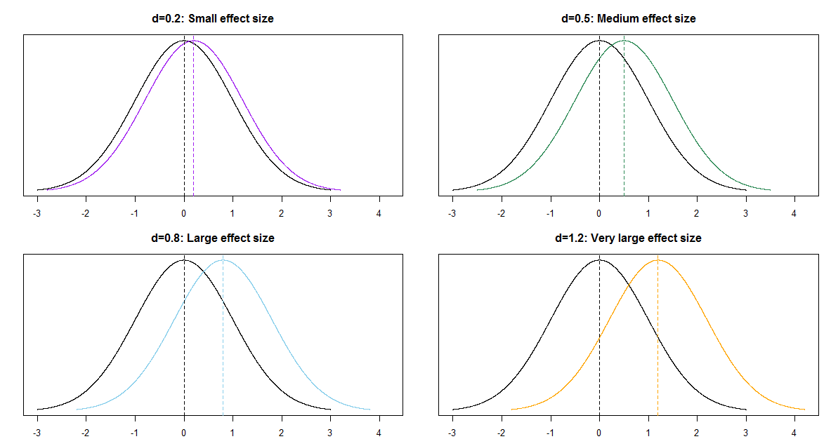
Some rough guidelines for interpreting $|d|$:

d	0.2	0.5	0.8	1.2	2.0
Effect size	Small	Medium	Large	Very Large	Huge

For example, assume the two population distributions are Normal and the two population standard deviations are equal. Then when the effect size is 1.0 the median of the distribution with the higher mean is the 84th percentile of the distribution with the lower mean, which is a very large difference.

d	0.2	0.5	0.8	1.0	1.2	2.0
Effect size	Small	Medium	Large		Very Large	Huge
Median of population 1 is
(blank) percentile of population 2	58th	69th	79th	84th	89th	98th

Notes on the JAGS code.

You should be able to define the prior parameters for the Multivariate Normal distribution within JAGS, but I keep getting an error. So I’m defining prior parameters outside of JAGS and then passing them in with the data. (I can never remember what you can do in JAGS and what you need to do in R and pass to JAGS.)
The Bivariate Normal prior is coded in JAGS using dmnorm.vcov which has two parameters: a mean vector and a covariance matrix. (There is also dmnorm is which is parametrized by the precision matrix.)
The prior mu[1:2] ~ dmnorm(...) creates a vector mu with two components mu[1] and mu[2]. When "mu" is called in the variable.names = c("mu", "sigma") argument of coda.samples JAGS will return the vector mu — that is, both components mu[1] and mu[2]. See the output of posterior_sample.
Group variables (like non-smoker/smoker) need to be coded as numbers in JAGS, starting with 1. So x recodes smoking status as 1 for non-smokers and 2 for smokers.
We have data on individual birthweights, so we evaluate the likelihood of each individual value y[i] using a Normal distribution and then use a for loop to find the likelihood for the sample.
Notice that the mean used in the likelihood depends on the group: mu[x[i]]. For example, if element i has birthweight y[i] = 8 and is a non-smoker x[i] = 1, then the likelihood is evaluated using a Normal distribution with mean $\mu_1$; for this element y[i] ~ dnorm(mu[x[i]], ...) in JAGS is like calling dnorm(y[i], mu[x[i]], ...) = dnorm(8, mu[1], ...) in R. If element i has birthweight y[i] = 7.3 and is a smoker x[i] = 2, then the likelihood is evaluated using a Normal distribution with mean $\mu_2$; for this element y[i] ~ dnorm(mu[x[i]], ...) in JAGS is like calling dnorm(y[i], mu[x[i]], ...) = dnorm(7.3, mu[2], ...) in R.
The variable.names = c("mu", "sigma") argument of coda.samples tells JAGS which simulation output to save. Given the joint posterior distributon of the primary parameters, it is relatively easy to obtain the posterior distribution of transformations of these parameters outside of JAGS in R.

Non-Normal Likelihood

The sample data exhibits a long left tail, similar to what we observed in the previous chapter. Therefore, a non-Normal model might be more appropriate for the distribution of birthweights. The code and output below uses a $t$-distribution for the likelihood, similar to what was done in the previous section. The posterior distribution of $(\mu_1, \mu_2)$ is fairly similar to what was computed above for the model with the Normal likelihood. The model below based on the $t$-distribution likelihood shifts posterior credibility a little more towards mean birthweights for non-smokers being greater than birthweights for smokers. But the difference is still small in absolute terms; at most 0.5 pounds or so. In terms of comparing population means, the choice of likelihood (Normal versus $t$) does not make much of a difference in this example. That is, the inference regarding $\mu_1 - \mu_2$ appears not to be too sensitive to the choice of likelihood. However, if we were using the model to predict birthweights, then the $t$-distribution based model might be more appropriate, as we observed in the previous chapter.

# Model
model_string <- "model{

  # Likelihood
  for (i in 1:n){
      y[i] ~ dt(mu[x[i]], 1 / sigma ^ 2, tdf)
  }

  # Prior
  mu[1:n_groups] ~ dmnorm.vcov(mu_prior_mean[1:n_groups],
                               mu_prior_cov[1:n_groups, 1:n_groups])

  sigma ~ dgamma(1, 1)
  
  tdf <- 1 + tdf0

  tdf0 ~ dexp(1 / 29)

}"

dataList = list(y = y, x = x, n = n, n_groups = n_groups,
                mu_prior_mean = mu_prior_mean, mu_prior_cov = mu_prior_cov)

# Compile
Nrep = 10000

n.chains = 5

model <- jags.model(textConnection(model_string),
                    data = dataList,
                    n.chains = n.chains)

## Compiling model graph
##    Resolving undeclared variables
##    Allocating nodes
## Graph information:
##    Observed stochastic nodes: 999
##    Unobserved stochastic nodes: 3
##    Total graph size: 2020
## 
## Initializing model

# Simulate
update(model, 1000, progress.bar = "none")

posterior_sample <- coda.samples(model,
                                 variable.names = c("mu", "sigma", "tdf"),
                                 n.iter = Nrep,
                                 progress.bar = "none")


sim_posterior = as.data.frame(as.matrix(posterior_sample))
names(sim_posterior) = c("mu1", "mu2", "sigma", "tdf")
head(sim_posterior)

##     mu1   mu2 sigma   tdf
## 1 7.285 6.945 1.063 4.352
## 2 7.303 6.880 1.096 3.928
## 3 7.326 6.890 1.041 4.429
## 4 7.339 6.912 1.148 4.914
## 5 7.376 6.929 1.102 4.531
## 6 7.369 6.922 1.066 3.930

ggplot(sim_posterior, aes(mu1, mu2)) +
  geom_point(color = "seagreen", alpha = 0.4) +
  stat_ellipse(level = 0.98, color = "black", size = 2) +
  stat_density_2d(color = "grey", size = 1) +
  geom_abline(intercept = 0, slope = 1)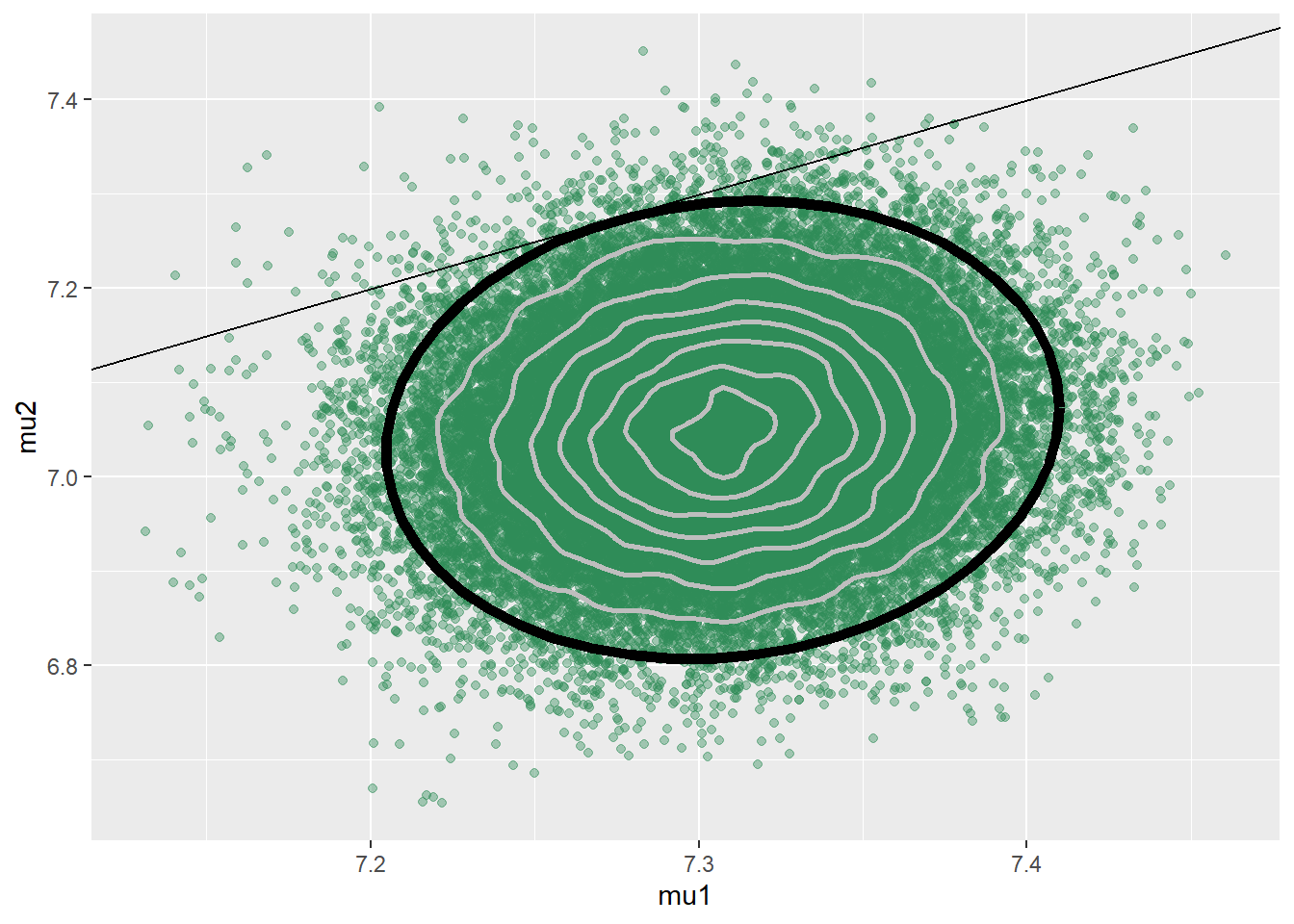

ggplot(sim_posterior, aes(mu1, mu2)) +
  stat_density_2d(aes(fill = ..level..),
              geom = "polygon", color = "white") +
 scale_fill_viridis_c() +
  geom_abline(intercept = 0, slope = 1)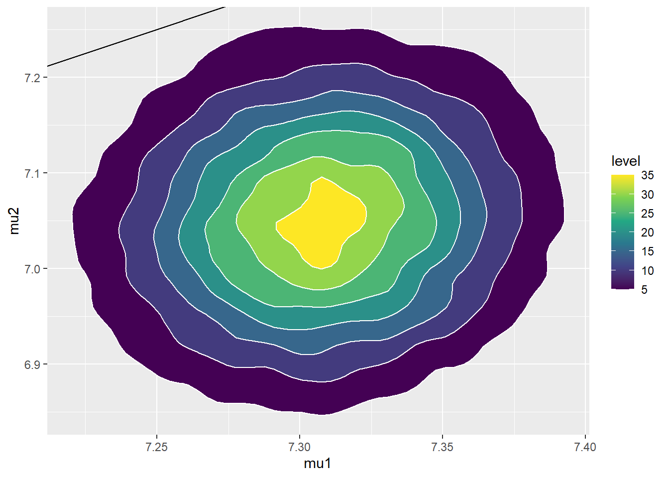

cor(sim_posterior$mu1, sim_posterior$mu2)

## [1] 0.09826

sim_posterior = sim_posterior %>%
      mutate(mu_diff = mu1 - mu2)

ggplot(sim_posterior,
       aes(mu_diff)) +
  geom_histogram(aes(y=..density..), color = "black", fill = "white") +
  geom_density(size = 1, color = "seagreen") +
  labs(x = "Difference in population mean birthweight (pounds, non-smokers - smokers)",
       title = "Posterior Distribution")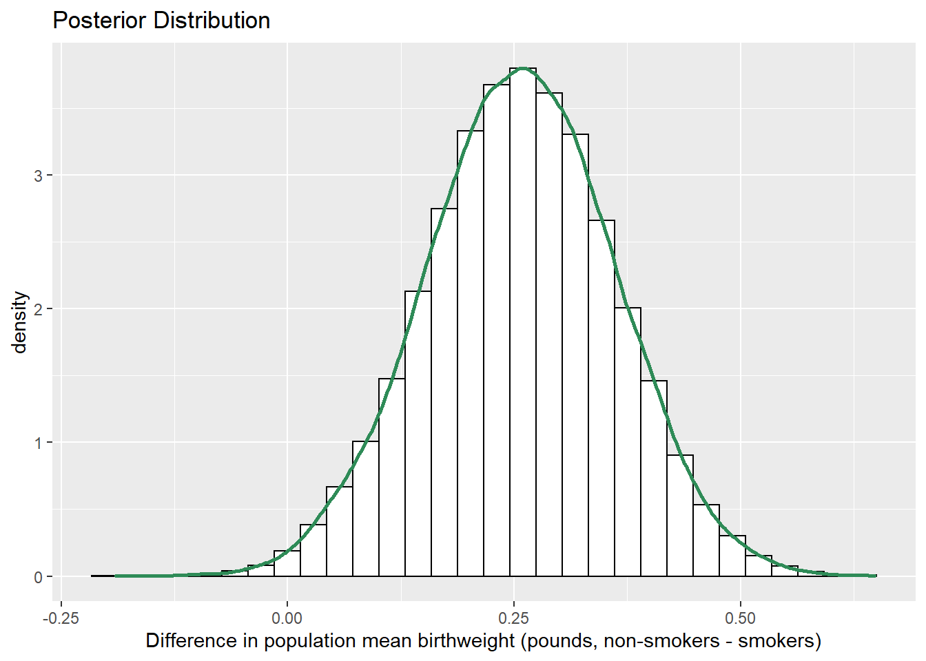

quantile(sim_posterior$mu_diff, c(0.01, 0.10, 0.25, 0.75, 0.90, 0.99))

##      1%     10%     25%     75%     90%     99% 
## 0.01584 0.12313 0.18665 0.32746 0.39013 0.49700

sum(sim_posterior$mu_diff > 0 ) / length(sim_posterior$mu_diff)

## [1] 0.9937