8.1 A brief review of continuous distributions

This section provides a brief review of continuous probability distributions. Throughout, $U$ represents a continuous random variable that takes values denoted $u$. In a Bayesian framework, $u$ can represent either values of parameters $\theta$ or values of data $y$.

The probability distribution of a continuous random variable is (usually) specified by its probability density function (pdf) (a.k.a., density), usually denoted $f$ or $f_U$. A pdf $f$ must satisfy: \[\begin{align*} f(u) &\ge 0 \qquad \text{for all } u\\ \int_{-\infty}^\infty f(u) du & = 1 \end{align*}\] For a continuous random variable $U$ with pdf $f$ the probability that the random variable falls between any two values $a$ and $b$ is given by the area under the density between those two values. \[ P(a \le U \le b) =\int_a^b f(u) du \] A pdf will assign zero probability to intervals where the density is 0. A pdf is usually defined for all real values, but is often nonzero only for some subset of values, the possible values of the random variable. Given a specific pdf, the generic bounds $(-\infty, \infty)$ should be replaced by the range of possible values, that is, those values $u$ for which $f(u)>0$.

For example, if $U$ can only take positive values we can write its pdf as \[ f(u) = \begin{cases} \text{some function of $u$}, & u>0,\\ 0, & \text{otherwise} \end{cases} \] The “0 otherwise” part is often omitted, but be sure to specify the range of values where $f$ is positive.

The expected value of a continuous random variable $U$ with pdf $f$ is \[ E(U) = \int_{-\infty}^\infty u\, f(u)\, du \]

The probability that a continuous random variable $U$ equals any particular value is 0: $P(U=u)=0$ for all $u$. A continuous random variable can take uncountably many distinct values, e.g. $0.500000000\ldots$ is different than $0.50000000010\ldots$ is different than $0.500000000000001\ldots$, etc. Simulating values of a continuous random variable corresponds to an idealized spinner with an infinitely precise needle which can land on any value in a continuous scale.

A density is an idealized mathematical model for the entire population distribution of infinitely many distinct values of the random variable. In practical applications, there is some acceptable degree of precision, and events like “X, rounded to 4 decimal places, equals 0.5” correspond to intervals that do have positive probability. For continuous random variables, it doesn’t really make sense to talk about the probability that the random value equals a particular value. However, we can consider the probability that a random variable is close to a particular value.

The density $f(u)$ at value $u$ is not a probability But the density $f(u)$ at value $u$ is related to the probability that the random variable $U$ takes a value “close to $u$” in the following sense \[ P\left(u-\frac{\epsilon}{2} \le U \le u+\frac{\epsilon}{2}\right) \approx f(u)\epsilon, \qquad \text{for small $\epsilon$} \] So a random variable $U$ is more likely to take values close to those with greater density.

In general, a pdf is often defined only up to some multiplicative constant $c$, for example \[\begin{align*} f(u) & = c\times\text{some function of $u$}, \quad \text{or}\\ f(u) & \propto \text{some function of $u$} \end{align*}\]

The constant $c$ does not affect the shape of the density as a function of $u$, only the scale on the density (vertical) axis. The absolute scaling on the density axis is somewhat irrelevant; it is whatever it needs to be to provide the proper area. In particular, the total area under the pdf must be 1. The scaling constant is determined by the requirement that $\int_{-\infty}^\infty f(u)du = 1$. (Remember to replace the generic $(-\infty, \infty)$ bounds with the range of possible values.)

What is important about the pdf is relative height. For example, if two values $u$ and $\tilde{u}$ satisfy $f(\tilde{u}) = 2f(u)$ then $U$ is roughly “twice as likely to be near $\tilde{u}$ than $u$” \[ 2 = \frac{f(\tilde{u})}{f(u)} = \frac{f(\tilde{u})\epsilon}{f(u)\epsilon} \approx \frac{P\left(\tilde{u}-\frac{\epsilon}{2} \le U \le \tilde{u}+\frac{\epsilon}{2}\right)}{P\left(u-\frac{\epsilon}{2} \le U \le u+\frac{\epsilon}{2}\right)} \]

$Illustration of $P(1<U<2.5)$ (left) and $P(0.995<U<1.005)$ and $P(1.695<U<1.705)$ (right) for $U$ with an Exponential(1) distribution, with pdf $f_U(u) = e^{-u}, u>0$. The plot on the left displays the true area under the curve over (1, 2.5). The plot on the right illustrates how the probability that $U$ is “close to” $u$ can be approximated by the area of a rectangle with height equal to the density at $u$, $f_U(u)$. The density height at $u=1$ is twice as large than the density height at $u=1.7$, so the probability that $U$ is “close to” 1 is (roughly) twice as large as the probability that $U$ is “close to” 1.7.$ $Illustration of $P(1<U<2.5)$ (left) and $P(0.995<U<1.005)$ and $P(1.695<U<1.705)$ (right) for $U$ with an Exponential(1) distribution, with pdf $f_U(u) = e^{-u}, u>0$. The plot on the left displays the true area under the curve over (1, 2.5). The plot on the right illustrates how the probability that $U$ is “close to” $u$ can be approximated by the area of a rectangle with height equal to the density at $u$, $f_U(u)$. The density height at $u=1$ is twice as large than the density height at $u=1.7$, so the probability that $U$ is “close to” 1 is (roughly) twice as large as the probability that $U$ is “close to” 1.7.$

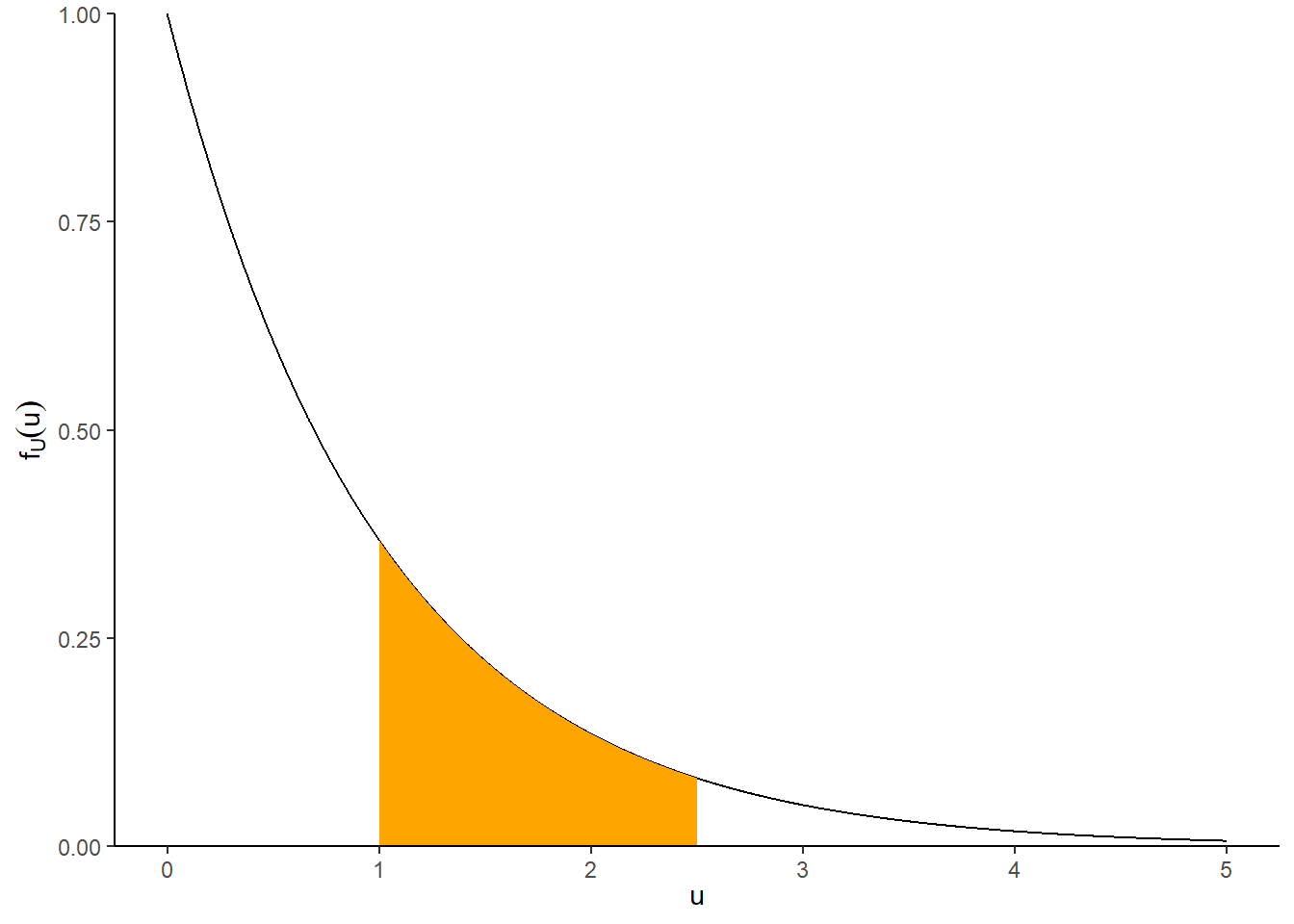
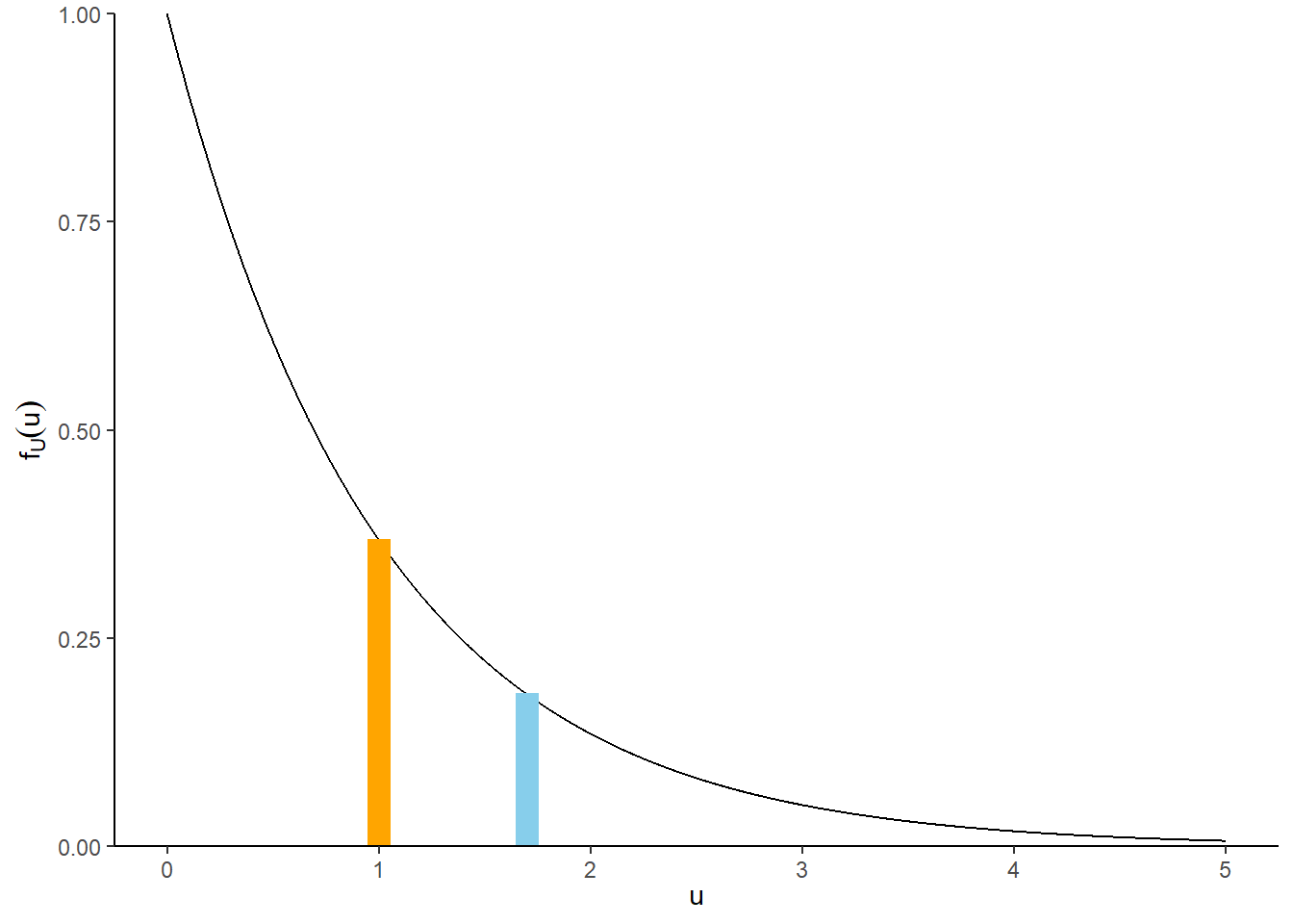
Figure 8.1: Illustration of $P(1<U<2.5)$ (left) and $P(0.995<U<1.005)$ and $P(1.695<U<1.705)$ (right) for $U$ with an Exponential(1) distribution, with pdf $f_U(u) = e^{-u}, u>0$. The plot on the left displays the true area under the curve over (1, 2.5). The plot on the right illustrates how the probability that $U$ is “close to” $u$ can be approximated by the area of a rectangle with height equal to the density at $u$, $f_U(u)$. The density height at $u=1$ is twice as large than the density height at $u=1.7$, so the probability that $U$ is “close to” 1 is (roughly) twice as large as the probability that $U$ is “close to” 1.7.

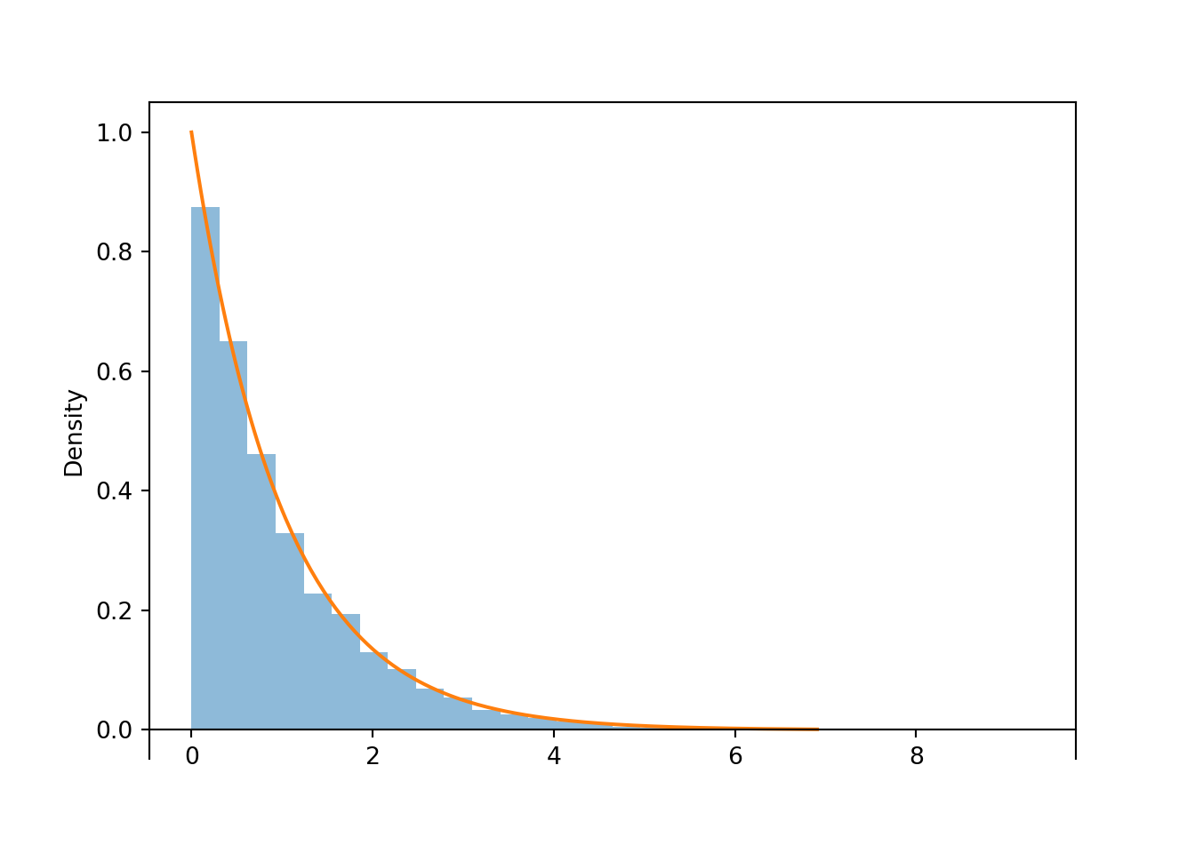
A sample of values of a continuous random variable is often displayed in a histogram which displays the frequencies of values falling in interval “bins”. The vertical axis of a histogram is typically on the density scale, so that areas of the bars correspond to relative frequencies.